
1. Introduction
Increases in impervious surface from development subsequently increase rates of stormwater runoff draining into receiving channels and downstream watersheds (Canters et al. 2006; Wang et al. 2017, 2023). Since land conversion and development continue apace in the United States, the impact of increasing impervious surface due to urbanization is a critical issue (Roberts et al. 2009) leading to extensive erosion of receiving channels, habitat degradation, and water quality impairments downstream (Bedi et al. 2015). Urbanizing watersheds are susceptible to erosion from stormwater runoff as greater discharges strip away sediment, often deepening receiving channels to accommodate increased velocities and volumes of runoff (Dindinger et al. 2020). Common mitigation measures, or Best Management Practices (BMPs), include ponds meant to slow rates of discharge into receiving channels to limit the pace of erosion (Hancock et al. 2010; Cronshey et al. 1986).
Stormwater retention ponds sizing determines the discharge rates entering receiving channels and thus strongly influences channel geomorphology and water quality (Cronshey et al. 1986). To support the design process, Technical Release 55 (TR-55), a method established by the United States Department of Agriculture (USDA) in 1986, models pre- and post-development peak discharges (Cronshey et al. 1986; Ormsbee et al. 2020). TR-55 is an embedded functionality within HydroCAD stormwater modeling software, providing simplified procedures to estimate stormwater runoff volumes, peak discharge hydrographs, and storage volumes for small, urbanizing watersheds in the United States. Prior sensitivity analyses conducted on TR-55 have found that peak discharges can be sensitive to Curve Numbers (CN) and Time of Concentration (Tc) (Shi & Wang 2020; Soomro et al. 2019; Yogi et al. 2021). CNs predict runoff volume by calculating potential maximum retention, S, in Equation 1. Initial abstraction is also derived using S, whereas rainfall is a user-defined parameter in Equation 1. Although this study examined Ia/S ratios ranging from 0.01 – 0.20, peak discharge sensitivity over realistic Ia/S variation (0.15 – 0.20) was moderate at New Kent (~18% increase in peak discharge rates [Qp]) and larger at Cow Swamp (~140% increase in Qp), providing a quantitative basis for deemphasizing Ia/S relative to Hydrologic Soil Group (HSG) effects (Figure S1). CNs remain the primary determinant of runoff volume, and inaccuracies can result in unreliable peak discharge predictions (Tan et al. 2018; Ormsbee et al. 2020; Shi & Wang 2020; Munna et al. 2021). Tc (Equation 2), the time it takes for water at the most hydraulically distant point in a watershed to travel to a point of interest in the same watershed, includes 3 different types of flow: (1) sheet flow, for which its common to use a maximum of 300 ft, (2) shallow concentrated flow, and (3) channel flow (Cronshey et al. 1986, Venkata Ramana 2014; Adalikwu and Burckhard 2021). Because Tc directly controls the shape and timing of the hydrograph, assumptions about sheet flow length influence predicted peak discharge. In addition, CNs and Tc are influenced by soil classifications based on infiltration rates, known as HSGs (Cronshey et al. 1986; Mockus et al. 2007). These classifications include “A” (excellent infiltration rates; lowest runoff), “B” (good), “C” (fair), and “D” (poor infiltration rates; highest runoff) (Cronshey et al. 1986; Mockus et al. 2007). Because both CN and Tc depend directly on HSGs, errors in soil classification can propagate through TR-55/HydroCAD and substantially alter peak discharge predictions.
$$Q = \frac{\left( P - I_{a} \right)^{2}}{\left( P - I_{a} \right) + S}\hspace{2em} (1)$$
Where:
Q = runoff (in)
P = rainfall (in)
S = potential maximum retention after runoff begins (in)
Ia = initial abstraction (in)
Tc = Tt1 + Tt2 + … Ttm (2)
Although a wealth of scientific literature addresses stormwater and BMP modeling, design, and performance, a clear gap remains regarding the commonly used stormwater modeling software HydroCAD and the potential for user error when sizing retention ponds. To address this gap, the goal of this study was to compare HydroCAD model outputs (e.g., Qp), to field measurements and evaluate the influence of key parameters, including HSGs, CNs, and Tc, on those outputs. Specifically, this study aimed to: (1) evaluate the sensitivity of Qp to changes in HSG classifications, and (2) assess whether the TR-55 maximum sheet flow distance of 91.4 m (300 ft) aligns with realistic site behavior. Analyses were conducted using data from 2 study sites located in James City County, Virginia, United States, and New Kent County, Virginia, United States.
2. Materials and Methods
2.1. Study Sites
Success of retention ponds in moderating stormwater flows can be varied. What has been coined by residents of Williamsburg, Virginia, United States, as the “Grand Canyon,” and serves as the project impetus for this study, is a severely incised channel 7.62 m (25 ft) in depth located immediately downstream from a stormwater retention pond in the coastal plain of Virginia, United States. The resulting erosion illustrates an extreme outcome from incorrectly designed stormwater ponds (Daily Press 2024). Estimates of pre- and post-development peak discharges guide the sizing of these BMPs, where under- or over-estimated peak discharges can lead to stormwater pond designs that do not retain or release runoff similar to pre-development rates (Cronshey et al. 1986). In this example from Virginia, erosion of stream and riparian natural habitat has impaired the overall environmental quality of this waterway. As of fall 2025, the Virginia Department of Transportation (VDOT) has spent $2.25M for stream and floodplain restoration to stabilize and regrade the reach to protect roads and other infrastructure due to the extensive headward erosion (Daily Press 2024).
Two study sites were selected in James City County, Virginia, United States, and New Kent County, Virginia, United States (Figure 1). Both sites are predominantly wooded and undeveloped, with minimal impervious surfaces and similar soil and topographic characteristics. These locations were chosen for accessibility and because their undeveloped status provides conditions likely to challenge HydroCAD modeling assumptions, particularly for TR-55 Qp estimates.
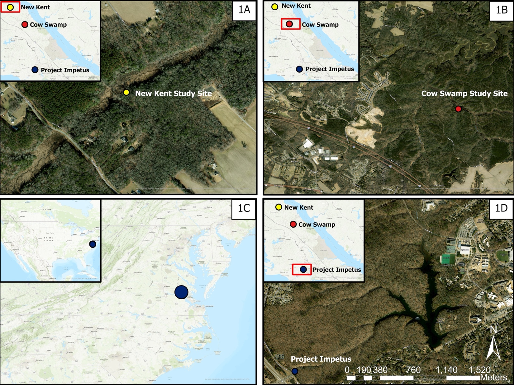
Fig 1. Aerial imagery of the 2 study sites with respect to the Chesapeake Bay, Virginia, United States, and the greater United States. (A) New Kent site in New Kent County, Virginia; (B) Cow Swamp site in James City County, Virginia; (C) Continental United States showing study region; (D) Regional context showing site location within the Chesapeake Bay watershed. Maps data: Esri 2025, Maxar, Earthstar Geographics, TomTom, Garmin, FAO, NOAA, USGS, ©OpenStreetMap contributors, CGIAR, and the GIS User Community (Esri 2025a, 2025b).
The study was conducted at New Kent (New Kent County, Virginia) and Cow Swamp (James City County, Virginia). The New Kent site (Figure 2) consisted of ~50% mixed agricultural and ~50% wooded land, with a drainage area of 328,754 m², while Cow Swamp was 100% wooded with a drainage area of 320,000 m². Soil types were classified based on USDA soil maps: New Kent was primarily HSG C and HSG D (69.3%), and Cow Swamp was primarily HSG B (53.8%) (Table 1). Flow monitoring equipment installed at both sites recorded water levels during rainfall events used for both modeling and hand-calculated peak discharge comparisons.
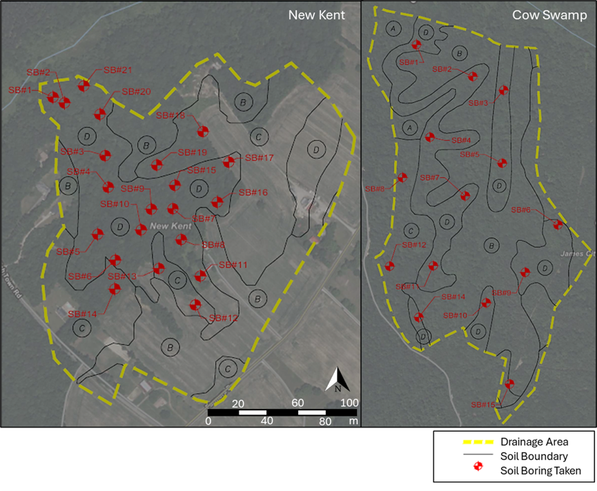
Fig. 2. Maps of the New Kent (A) and Cow Swamp (B) study sites showing delineated drainage areas, soil boring locations, and hydrologic soil group (HSG) distributions based on USDA soil maps. Soil contours highlight spatial variability in mapped HSG classifications, which were later compared with field-verified soil samples. Map data: Google Earth 2025, USDA Web Soil Survey 2019, County of New Kent GIS 2024, James City County GIS 2024 (Google Earth 2025a, 2025b; USDA & NRCS 2019; County of New Kent n.d.; James City County 2024).
Table 1 Distribution of hydrologic soil groups (HSGs) at the New Kent and Cow Swamp study sites. Areas and percentages are reported for each HSG class, illustrating the spatial composition of soil types used in HydroCAD modeling and sensitivity analyses.
| HSGs | New Kent Area (m2) | New Kent Percentage (%) |
Cow Swamp Area (m2) | Cow Swamp Percentage (%) |
| A | 254 | 0.077 | 23,500 | 7.33 |
| B | 100,400 | 30.6 | 172,300 | 53.8 |
| C | 116,500 | 35.4 | 35,100 | 11.0 |
| D | 111,600 | 33.9 | 89,100 | 27.8 |
2.2. Field Measurements and Data Collection
Rainfall data were collected at each site using a standard manual rain gauge installed in an open area near each study site. Rainfall depth was recorded following each precipitation event and used to inform model inputs and contextualize hydrologic conditions during field measurement. Field measurements were used for 2 purposes: (1) to inform pre-development HydroCAD model inputs, improving accuracy beyond map-based data, and (2) to calculate pre-development peak discharge (Qp) manually using Manning’s equation.
2.2.1. Topographic Surveys
Topographic surveys were conducted using Leica Total Stations (868812 TS10 1” R1000) with a reflectorless R1000 Electronic Distance Measuring device and a standard surveyor’s prism pole. Accuracy of survey points was within ±0.0305 m. Horizontal and vertical control points were established in the field. After the installation of monitoring equipment, survey points were taken perpendicular to the streams, as well as upstream and downstream of sensor locations for generation of site cross-sections and profiles. Survey data were uploaded and post-processed in Carlson surveying software with AutoCAD using basic coordinate geometry: northings, eastings, elevations, (x, y, z). Profiles informed HydroCAD reach geometry and were also used to calculate cross-sectional area (A) and wetted perimeter (P), which were needed to compute hydraulic radius (R = A / P) for peak discharge calculations.
2.2.2. Soil Sampling
Soil borings were randomly collected only in areas mapped as HSG C and HSC D at each site (Figure 3). These groups were prioritized because misclassification would have a greater impact on runoff estimates: if “C” or “D” are mistakenly identified, pre-development Qp values may be overestimated, leading to less accurate and potentially more harmful design outcomes. In contrast, errors in “A” or “B” soils are less critical, as they naturally generate lower runoff rates and thus provide more realistic estimates in undeveloped, wooded environments. Collection of samples was done using an 8.255-cm (3.25-in) auger. Two samples per borehole were taken: 0 cm – 66 cm (0 in – 26 in) and 66 cm – 116 cm (26 in – 46 in) following National Engineering Handbook guidelines (Mockus et al. 2007). Samples were analyzed at Landtech Resources Inc. following ASTM D2488. An Authorized Onsite Soil Evaluator and Licensed Professional Soil Scientist (VA #0345) verified classifications. Soil data were used to refine HydroCAD CNs. Initial model runs used map-based HSG data, and subsequent runs incorporated measured soils, with outputs compared for accuracy.
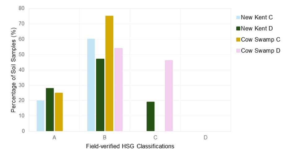
Fig. 3. Comparison of USDA soil map classifications (“C” and “D”) and field-verified HSGs at the New Kent and Cow Swamp sites. Grouped bars show the proportion of C- and D-classified soils that were found to be A, B, C, or D, based on soil borings, highlighting the extent of misclassification in the baseline soil maps.
2.2.3. Flow Monitoring
Water level and velocity were recorded May 2023 through October 2023 in a stream at each site using a MantaRay Portable Ultrasonic Flow Monitor (Greyline Instruments, Massena, New York, United States), which uses a submerged ultrasonic sensor to measure flow in open channels. Water level sensors collected continuous data at 5-minute intervals throughout the monitored storm event, which resulted in one storm event analyzed per site due to study timeframe constraints. These data were used to validate HydroCAD simulations and provide observed water elevations and velocities for the manually calculated peak discharge.
2.3. HydroCAD Modeling
Since only pre-development peak discharges were modeled, one subcatchment per site (i.e., drainage area) was defined in HydroCAD. CNs for each site were based on acreage per HSG, for which all 4 soil classifications were present. Area per HSG was determined through available soil contours and classifications were later corrected based on retrieved soil samples. Tc values were set according to flow characteristics, with undeveloped wooded areas consisting predominately of sheet flow. Reaches were created using field-surveyed cross-section points and elevations. Rainfall was measured directly using site-installed gauges and daily totals (6.4 cm) were distributed in HydroCAD using an NRCS Type II 24-hour curve. HydroCAD generated hydrographs, which were analyzed for Qp, and compared to independent calculations for validation.
Topographic contours and soil data were obtained from county GIS parcel viewers (James City County 2024; County of New Kent n.d.) and USDA Web Soil Survey (USDA & NRCS 2019), then imported into AutoCAD to verify drainage areas. VADEQ recommendations, based on the Virginia Runoff Reduction Method (VRRM) and Virginia Administrative Code (9VAC25-875-600 E), were applied for cover type conditions, where wooded, undeveloped areas are classified as “good” cover type for all HSGs (Center for Watershed Protection & Chesapeake Stormwater Network 2008; Virginia Administrative Code 2024a).
Sensitivity analyses followed established practices for evaluating parameter uncertainty and model responsiveness in CN-based hydrologic modeling frameworks (Ponce & Hawkins 1996). A series of sensitivity analyses were performed by varying HSGs (5 iterations per site), CNs (5 iterations per site), and sheet flow lengths (30 iterations per site). For soil sensitivity, scenarios included baseline USDA soil map HSGs, field-verified HSGs from soil borings, and uniform HSG assignments (All A, All B, All C, and All D). Hydrographs from multiple runs were exported for analysis in Microsoft Excel and RStudio. For sheet flow sensitivity, flow lengths were varied from 3.048 m to 91.4 m while holding all other inputs constant. Relationships between sheet flow length and Qp were assessed using second-order polynomial regression to capture nonlinear runoff responses commonly served in hydrologic systems (Mockus et al. 2007). Percent changes in Qp relative to baseline conditions were calculated to quantify sensitivity to model parameters.
2.4. Peak Discharge Calculations
Field measurements were used to calculate pre-development Qp for each site, both for model validation and for direct comparison to hand-calculated values. Two complementary approaches were used: (1) stream discharge using Manning’s equation, consistent with procedures outlines in TR-55 for sheet and shallow concentrated flow (Cronshey et al. 1986, Mockus et al. 2007) and (2) drainage area peak flow using the flow rate equation, which relates watershed characteristics, time of concentration, and rainfall depth to peak flow estimates (Cronshey et al. 1986, Mockus et al. 2007).
Manning’s equation was applied to each surveyed stream cross-section to calculate flow in the channel (Equation 3). Manning’s roughness coefficient of 0.40 for sheet flow in wooded areas, provided from TR-55 reference table, was used at each site. This coefficient was based on observed site conditions characterized by dense vegetation and surface roughness, consistent with values reported in TR-55 and established guidance for natural surfaces (Cronshey et al. 1986).
$$Q = \left( \frac{1.49}{n} \right)\text{AR}^{\frac{2}{3}}\sqrt{S}\hspace{2em} (3)$$
Where:
Q = Discharge \(\left( \frac{m^{3}}{s} \right)\)
n = Manning’s Roughness Coefficient
A = Flow area (m2)
R = Hydraulic radius (m)
S = Channel slope \(\left( \frac{m}{m} \right)\)
Topographic survey data provided A and P, while flow monitoring sensors supplied water level measurements to define flow depth during storm events. The discharge calculation yielded peak flow rates in the stream channel that were compared to HydroCAD outputs to assess model performance.
The peak discharge of the entire drainage area was estimated using the flow-rate equation (Equation 4), where A was derived from the topographic surveys and Q was derived from the in-stream flow monitors.
Q = vA (4)
Where:
Q = Discharge \(\left( \frac{m^{3}}{s} \right)\)
A = Cross-sectional vector area (m2)
By combining Manning-derived velocities with measured water levels, we calculated the total peak flow exiting the drainage area. These values were compared to HydroCAD outputs to assess model accuracy and sensitivity to soil, topography, and channel parameters. In total, we evaluated 3 groups of model runs in HydroCAD: baseline comparisons of mapped vs. field-verified soils, soil sensitivity tests with uniform HSG classifications, and sheet flow sensitivity analyses (Table 2).
Table 2 Summary of HydroCAD modeling scenarios used in sensitivity analyses. Each scenario group varied specific TR-55 parameters—Hydrologic Soil Groups (HSGs), Curve Numbers (CNs), or sheet flow length—to evaluate their influence on time of concentration (Tc) and peak discharge (Qp).
| Scenario Group | Parameters Varied | Purpose |
| HSG’s influence on modeled Qp | USDA soil map HSG classification vs. field-verified HSG classification |
Compare standard HydroCAD inputs with site-specific soil data and its effect on Qp |
| CN sensitivity to HSGs |
Hypothetical uniform HSGs (all A, B, C, and D) |
Test sensitivity of Qp to soil group classifications |
| Sheet Flow Sensitivity | Sheet flow lengths from 3.048 m – 81.4 m (increments of 10) |
Evaluate TR-55’s 91.4 m sheet flow assumption on Tc and its effect of Qp |
3. Results
3.1. Soil Samples
At both sites, 0% of the soil samples collected from sections of “D” classified soil were found to be representative of “D” HSG classifications. Similar misrepresentations were identified across both sites for “C” classified soils, where 0% of “C” classified soil for New Kent and Cow Swamp were found to be representative of a “C” HGS classification. Most notably, of the soil borings taken, 60% of “C” designated soil at New Kent was actually “B” soil and 75% of “C” designated soil at Cow Swamp was “B” soil. Overall, “C” and “D” classified samples were more representative of either “B” or “A” HSG classifications (Figure 3; Table S2).
3.2. HydroCAD Modeling Scenarios
For the New Kent site using a Type II 24-hr observed rainfall event of 6.4 cm and USDA soil map HSG classifications, a HydroCAD Qp of 0.81 m3/s can be observed (Figure 4). Alteration of HSG classifications within the model, from majority “C” and “D” classifications to majority “B” and “A” classifications based on site soil samples, decreased Qp to 0.10 m3/s, approximately 8.1 times smaller than what was initially modeled. The Qp calculated using direct measurements was 0.11 m3/s with a stream discharge of 0.217 m3/s. The direct measurements and the HSG-adjusted model both show Qp is overestimated using USDA soil map data by approximately 640% and 710%, respectively. Additionally, the estimated total volume using the model outputs associated with USDA soil maps was approximately 7,600 m3/s, whereas the estimated total volume using site collected data was 800 m3/s, an overestimation by a factor of 9.5.
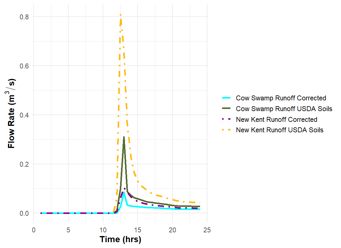
Fig. 4. Comparison of HydroCAD model Qp outputs for the New Kent study and Cow Swamp study sites. HydroCAD model using New Kent Runoff USDA Soils (yellow) had a Qp of 0.81 m3/s. New Kent Runoff Corrected (purple) using HSG classifications from site samples had a Qp of 0.10 m3/s. HydroCAD model using Cow Swamp Runoff USDA Soils (green) had a Qp of 0.31 m3/s. Cow Swamp Runoff Corrected (blue) using HSG classifications from site samples had a Qp of 0.09 m3/s.
At the Cow Swamp site, a Type II 24-hour rainfall event of 6.4 cm and USDA soil map HSG classifications yielded a HydroCAD Qp of 0.31 m3/s (Figure 4). Adjusting HSG classifications based on soil samples reduced Qp to 0.09 m3/s, 3.4 times smaller than the original model output. Using the direct measurements, Qp was calculated at 0.14 m3/s, with a stream discharge of 0.223 m3/s. The direct measurements and the HSG-adjusted model indicate the USDA soil maps overestimated Qp by approximately 120% and 240%, respectively. Similar to the New Kent site, the estimated total event discharge volume for Cow Swamp using the model outputs associated with USDA soil maps was approximately 2,200 m3, whereas the estimated total volume using site collected data was about 600 m3, an overestimation by a factor of 3.7.
Table 3 summarizes the modeled pre-development Qp for New Kent and Cow Swamp under baseline USDA soil maps HSGs, field-verified soils HSGs, uniform HSG sensitivity scenarios, and variations in minimum and maximum sheet flow length. This summary highlights the influence of soil classification and flow path length on modeled runoff and provides context for subsequent sensitivity analyses.
Table 3 Modeled HydroCAD peak discharge (Qp) for the New Kent and Cow Swamp study sites under different scenarios. Scenarios include baseline conditions using USDA soil map hydrologic soil groups (HSGs), field-verified soil HSGs, uniform HSG sensitivity analyses (All A and All D), and sheet flow length sensitivity analyses. Values illustrate the influence of soil classification and flow path length on Qp, highlighting the potential for over- or under-estimation of runoff depending on input assumptions.
| Scenario | Parameter Varied | New Kent Qp (m3/s) | Cow Swamp Qp (m3/s) | Notes |
| Baseline (USDA soils) |
HSG classification (map) | 0.81 | 0.31 | Default inputs |
| Field-verified soils | HSG classification (samples) | 0.10 | 0.09 | CN adjusted for soil borings |
| Soil sensitivity – All A | Uniform HSG | 0.01 | 0.00 | Lowest runoff potential |
| Soil sensitivity – All D | Uniform HSG | 1.25 | 2.22 | Highest runoff potential |
| Sheet flow sensitivity |
Sheet flow (3.048 m) | 33.82 | 24.55 | Tc minimized with default inputs |
| Sheet flow sensitivity |
Sheet flow (91.4 m) | 22.83 | 9.55 | Tc maximized with default inputs |
3.3. Sensitivity Analysis of HSG Influence on Qp
The biggest changes in Qp outputs were seen at both sites when comparing the Qp modeled with USDA soil maps to that modeled with corrected HSG conditions, and thereby varying CNs, based on site samples. Additionally, noticeable changes were observed when comparing the Qp modeled with USDA soil maps to the All A HSG and All D HSG conditions (Figure 5; Table 3). Sensitivity analyses for the New Kent and Cow Swamp sites indicate that baseline Qp outputs are highly sensitive to the extremes (“A” and “D”) of the HSG spectrum. Notably, the All C HSG condition produced very little change in Qp for New Kent, whereas Cow Swamp showed more pronounced changes. This difference is attributable to the baseline (USDA Soil Map) HSG distribution at each site. New Kent’s soils were classified predominately as “C” and “D” soil, therefore assigning all “C” results in minimal deviation from the baseline. Cow Swamp, on the other hand, was predominantly “B” soil, making the All “C” assumption more notable. A similar trend between the 2 sites can be observed in the All D HSG condition as well.
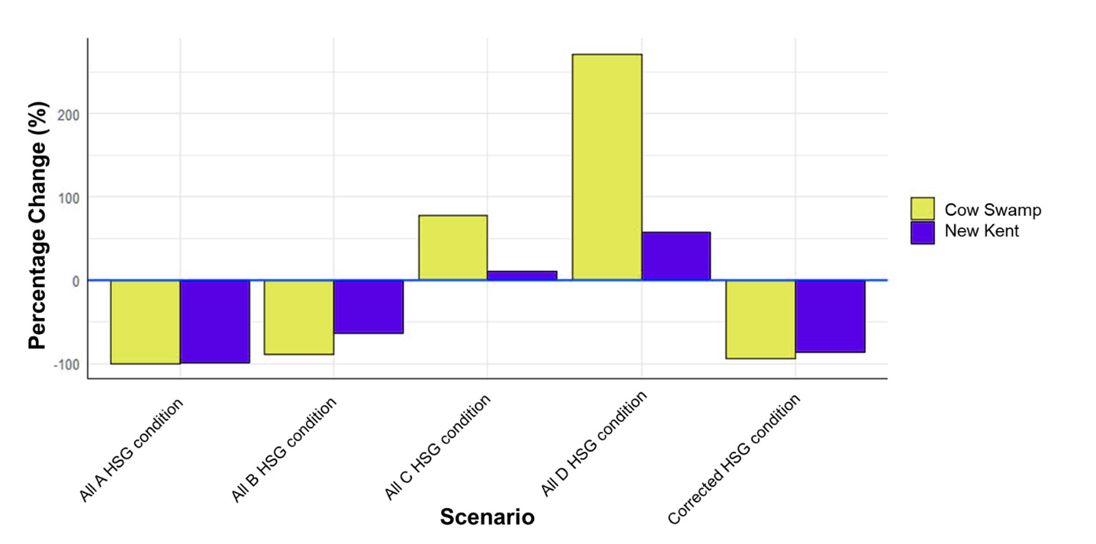
Fig. 5. Sensitivity analysis for the Cow Swamp and New Kent study sites. The X-axis shows different HSG scenarios and the Y-axis represents percentage change (%) of Qp. The solid blue line represents the baseline scenario (current USDA soil map conditions for both sites).
3.4. Sensitivity Analysis of Sheet Flow Length on Qp
Across both sites, sheet flow lengths were negatively correlated with respect to HydroCAD Qp (Figure S1; Table 3), indicating that shorter flow paths produce higher Qp values, whereas longer flow paths reduce Qp by increasing travel time and flow attenuation. Under baseline conditions, using USDA HSGs, only sheet flow lengths were varied to isolate their influence on modeled Qp. Increasing sheet flow length increases time of concentration by prolonging overland flow, thereby delaying watershed response and reducing peak discharge, consistent with NRCS TR-55 hydrologic theory. Alternative functional forms (linear and logarithmic) were explored during preliminary evaluation but did not adequately capture the observed non-linear relationship between sheet flow and Qp across the tested range. A second order polynomial regression was therefore selected and yielded a statistically significant relationship between sheet flow lengths and Qp for both sites (New Kent: df = 28, F-stat = 750.1, R2 = 0.997, adjusted R2 = 0.9963, p-value <0.05; Cow Swamp: df = 28, F-stat = 85.12, R2 = 0.94, adjusted R2 = 0.936, p-value <0.05).
4. Discussion
4.1. Parameter Influence on Qp
The Qp was demonstrably sensitive to changes in HSG, particularly to inaccuracies in applied soil classification. Soils misclassified as “C” or “D,” but more representative of “A” or “B,” led to overestimations of pre-development Qp. Thus, a model output that over-estimated pre-development Qp would cause a retention pond to be undersized, leading to excess stormwater discharge and downstream channel erosion. The HydroCAD model outputs using HSG classifications derived from USDA soil maps over-estimated pre-development Qp by approximately 710% for New Kent and 240% for Cow Swamp, relative to modeled outputs using HSG classifications from field samples.
The large discrepancies in modeled Qp, observed when using corrected HSGs, underscore the importance of accurate soil classification. HSGs are used to estimate infiltration rates via CNs, where group “A” soils are highly permeable, producing low runoff, while group “D” soils have poor permeability, producing high runoff. Post-development, additional impervious surfaces increase runoff relative to pre-development conditions. Retention ponds are sized based on the difference between pre- and post-development Qp. Therefore, if an undeveloped wooded area is classified primarily as “D” (low permeability soil), the difference in pre- and post-development runoff would be small, resulting in a smaller sized pond to catch the runoff. However, if that site was better represented as a “B” soil, the true pre-development Qp would be high, meaning a larger difference compared to post-development Qp, and therefore a larger pond would be needed. Misclassifying a site as a more permeable soil type can therefore drastically underestimate peak discharge, particularly for shorter flow paths where water concentrates quickly. These results highlight that even small errors in HSG assignment can propagate through hydrologic models, influencing stormwater management decisions. Due diligence to corroborate soil map accuracy is crucial for accurate HydroCAD results, as this study has highlighted a potential systemic issue in the application, warranting the need for further research.
When HSGs are misclassified, the effect on modeled runoff can be substantial. For example, consider a site that is mistakenly classified as consistently entirely or poorly drained soils (“D”). Under this misclassification, the pre-development Qp is estimated at 30 m3/s and the post-development Qp rises to 40 m3/s. Because the model difference is only 10 m3/s, the required retention pond would be relatively small. However, if the soils are correctly identified as well-drained (“B”), the pre-development Qp is about 5 m3/s. With post-development Qp still at 40 m3/s, the actual increase is 35 m3/s, meaning the retention pond must be designed much larger to safely manage stormwater. This example illustrates how misclassification can mask the true change in runoff and lead to undersized infrastructure.
4.2. Realistic Use of Sheet Flow Length
HydroCAD does not allow sheet flow lengths to exceed 91.4 m (300 ft), rejecting higher inputs. Considering the various model iterations and analysis of sheet flow lengths on Qp, a smaller sheet flow length results in a higher Qp, and potentially unrealistic pre-development representations. For example, using a smaller flow length of 30.5 m resulted in higher Qp outputs of 0.81 m3/s and 0.31 m3/s for New Kent and Cow Swamp, respectively. Using the maximum length of 91.4 m instead of the above example of 30.5 m lowered Qp outputs by approximately 22% and 48%, respectively. The sensitivity of Qp to flow length is not as severe in comparison to sensitivity to HSGs in the model but obviates the need for site inspections to discern sheet flow length as accurately as possible. Utilizing the 91.4 m maximum within HydroCAD, in tandem with accurate HSG classifications, will provide a more realistic output for undeveloped wooded areas that avoid the deleterious outcomes of overestimating pre-development Qp.
4.3. Regional Implications
Regulatory requirements varying by state, county, and municipality commonly demonstrate that post-development Qp for 2- and 10-year, 24-hour storms does not exceed pre-development Qp. In some cases, larger, 50- or 100-year, 24-hour storms are also modeled for flood controls. For example, Virginia’s state-level stormwater management standards suggest 1-, 2-, and 10-year, 24-hour storms should be used unless otherwise specified (Virginia Administrative Code 2024b).
The results of this study indicate that substantial discrepancies in modeled pre-development Qp can arise even under relatively typical rainfall events when key input parameters are mischaracterized. Such discrepancies raise concerns regarding the reliability of stormwater modeling conducted under current regulatory frameworks, as underestimated retention pond sizing may lead to increased discharge volumes, elevated erosion potential, and degraded downstream water quality.
Within the context of this study, the project impetus site drains into Lake Matoka, which ultimately contributes to the James River, a major tributary of the Chesapeake Bay. The 2022 Chesapeake Bay and watershed report card highlighted ongoing challenges across the watershed, with many tributaries exhibiting static or declining recovery trends (Vargas-Nguyen et al. 2023). Given that excess sedimentation remains a leading pollutant in U.S. waterways, ensuring that stormwater BMPs are appropriately sized to reflect true runoff conditions is critical for protecting receiving waters (U.S. EPA 2025).
Beyond environmental consequences, the financial implications of inadequate stormwater design can be substantial. For example, the ongoing VDOT restoration project associated with the project impetus site represents a cost of approximately $2.25 million (Kale 2024). Improved stormwater modeling practices may therefore reduce both ecological impacts and the long-term economic burdens associated with corrective restoration efforts.
4.4. National Implications
Proper modeling and management of stormwater runoff is a growing necessity, with the need for proper BMP design becoming more urgent as urbanization increases concomitant with increased rainfall intensities and amounts predicted from climate change models (Roy et al. 2008; Steinman et al. 2015; Sparkman et al. 2017). Since its nationwide adoption in 1986, TR-55 has remained a foundational method for stormwater modeling and is widely applied through software platforms such as HydroCAD.
This study demonstrates that modeled peak discharge using TR-55 based methods is highly sensitive CN, which is itself derived primarily from HSG classification. Although the modeling framework should be robust when properly parameterized, inaccuracies in input data, particularly soil classifications, can propagate through the model and result in substantial errors in predicted runoff.
While this analysis focuses on 2 coastal plain watersheds, the implications extend beyond the study area. USDA soil data sets, including the web soil survey, are routinely relied upon for stormwater modeling across the United States. These datasets explicitly note that mapped soil properties are intended for general planning purposes and should be verified through site-specific investigation. Despite these disclaimers, such data are often used without field validation and engineering practice. Continued reliance on misclassified HSGs has the potential to systematically underestimate or overestimate stormwater impacts, contributing to channel erosion and degradation of receiving waters at broader spatial scales. Taken together, these findings demonstrate the importance of careful evaluation of soil data inputs when implying TR-55-based methods nationwide. Improved attention to parameter accuracy, rather than changes to the modeling framework itself, represents a practical pathway for enhancing stormwater design outcomes across diverse watershed settings.
5. Conclusion
This study identified substantial inaccuracies in TR-55/HydroCAD predictions for undeveloped, wooded areas, primarily related to HSG classification. While these results are limited to one storm at each site, they highlight important limitations of current practice that may systematically affect BMP sizing and watershed outcomes. Broader, multi-event studies will be critical for fully assessing the scope of these limitations across differing land covers and regions. Our recommendations for the general enhancement of accuracy include 1) updating soil maps and 2) requiring soil analyses and site inspections (i.e., to confirm watershed boundaries, groundcover, and topography) prior to development. Specific recommendations for using HydroCAD to model undeveloped, wooded sites in good condition include1) eliminating the use of HSGs “C” and “D” to reduce the overall risk of overestimating pre-development Qp and 2) estimating sheet flow lengths obtained via site inspections and applying the 91.4 m (300 ft) maximum length for Tc calculations when applicable. These will produce more representative pre-development runoff rates.
Future work should focus on analyzing model outputs across various rainfall events at multiple undeveloped wooded sites in different regions. Studies comparing USDA soil maps to site soil analyses should also be conducted to identify the degree of potential discrepancies across various states. Lastly, these potential issues should be examined across different types of land cover (i.e., cultivated agricultural, grassland or pasture, fully developed, etc.) to determine if similar large systemic modeling errors may be occurring.
Supplementary Material
The online version of this article includes a link to a supplementary material file that contains the following supporting material: Table S1, Ia/S Ratio data for New Kent and Cow Swamp sites and their respective sensitivities; Table S2, Soil boring number, depth (cm), USDA HSG classification, and field sample classification of the soils taken from the New Kent and Cow Swamp study sites; Figure S1, Polynomial regression between various sheet flow lengths and Qp.
Acknowledgments
Funding for flow monitor equipment and use of surveying equipment was provided by Landtech Resources Inc. We would like to thank Barbara Beckingham and Scott Harris for all their help in the data collection and writing process. We would also like to thank Alex Russett, Chase Grogg, William Felts, and Ann Ruff for their generous assistance in the field and for providing expert engineering, surveying, and soils advice.
Author Contributions Statement
Conceptualization: BOC, MC; methodology: BOC, MC, WS; data analysis: BOC; writing original draft: BOC; review/editing original draft: RC, LK, WS; investigation: BOC; resources: MC; data curation: BOC; supervision: RC, LK, MC, WS. All authors have read and agreed to the published version of the manuscript.
Conflict of Interest Statement
The authors have no conflict of interest to report.
Data Availability Statement
Data from this study can be provided upon email request to the corresponding author.
Related Publication Statement
Earlier drafts of sections of this manuscript are included in the master’s thesis of the lead author at the College of Charleston.
Citation:
Ownby-Connolly B. 2024. Analyzing flaws in the use of stormwater modeling: Stormwater management implications for the Chesapeake Bay watershed. Charleston (SC): College of Charleston. https://www.proquest.com/openview/6ef33bd9f94534ab81bd1e553e270928/1?pq-origsite=gscholar&cbl=18750&diss=y
References
Adalikwu PA, Burckhard SR. 2021. How to resolve channel travel time errors in the TR-55 worksheet using Arc Hydro Tools, HEC-GeoHMS and HEC-HMS. Brookings (SD): South Dakota State University. https://openprairie.sdstate.edu/cgi/viewcontent.cgi?article=1002&context=cvlee_manual
Bedi M, Arora AS, Reddy AS. 2015. Quantification of the hydrological impacts of imperviousness in urban catchments using WIN TR-55. Int J Adv Technol Eng Sci. http://www.ijates.com/ADMIN/admin/postimages/images/fullpdf/1422367481_P551-557.pdf
Canters F, Chormanski J, Van De Voorde T, Batelaan O. 2006. Effects of different methods for estimating impervious surface cover on runoff estimation at catchment level [conference paper]. In: Painho M, Caetano M, editors. Proceedings of ACCURACY 2006 - 7th International Symposium on Spatial Accuracy Assessment in Natural Resources and Environmental Sciences; 2006 Jul 5-7; Lisbon, Portugal. Lisbon (Portugal): Instituto Geografico Portugues. p. 557-566.
Center for Watershed Protection, Chesapeake Stormwater Network. 2008. Technical memorandum: the runoff reduction method. Virginia Department of Environmental Quality. https://www.deq.virginia.gov/home/showpublisheddocument/15107/637908143151830000
County of New Kent. n.d. New Kent County CivQuest property site. [accessed 2026 Jun 17]. https://atlas.civ.quest/newkent_va
Cronshey R, McCuen R, Miller N, Rawls W, Robbins S, Woodward D. 1986. Urban hydrology for small watersheds TR-55. 210-VI-TR-55. 2nd ed. Washington (DC): USDA Natural Resources Conservation Service. https://www.hydrocad.net/pdf/TR-55%20Manual.pdf
Daily Press. 2024 Feb 21. Work on WMS Grand Canyon is underway. Newport News (VA): Daily Press. https://www.dailypress.com/2024/02/21/work-on-wms-grand-canyon-is-underway/
Dindinger J, Kyler K, Rockler A, Sample D, Fox L, Hughes S. 2020. Basic principles of watershed restoration and stormwater management in the Chesapeake Bay region. Virginia Cooperative Extension. https://cblpro.org/downloads/BasicPrinciplesWatershedRestoration.pdf
Esri. 2025a. World imagery [basemap]. Redlands (CA): Esri. [accessed 2026 Mar 6]. https://www.arcgis.com/home/item.html?id=10df2279f9684e4a9f6a7f08febac2a9
Esri. 2025b. World topographic map [basemap]. Redlands (CA): Esri. [accessed 2026 Mar 6]. https://www.arcgis.com/home/item.html?id=30e5fe3149c34df1ba922e6f5bbf808f
Google Earth. 2025a. 5600 Farmers Dr, Barhamsville, VA [satellite imagery]. Google Earth Pro V 7.3.7.1094. Mountain View (CA): Google. 37°28’41”N, 76°46’28”W. Image © 2025 Airbus. [accessed 2026 Mar 6]. https://earth.google.com
Google Earth. 2025b. [satellite imagery of James City County, Virginia]. Google Earth Pro V 7.3.7.1094. Mountain View (CA): Google. 37°25’31.5”N, 76°46’50.07”W. Image © 2025 Airbus. [accessed 2026 Mar 6]. https://earth.google.com
Hancock GS, Holley JW, Chambers RM. 2010. A field-based evaluation of wet retention ponds: how effective are ponds at water quantity control? J Am Water Resour Assoc. 46(6):1145–1158. https://doi.org/10.1111/j.1752-1688.2010.00481.x
HydroCAD. 2025. Solutions public. [accessed 2025 Sep 2]. https://www.hydrocad.net/solutions/public.htm
James City County. 2024. James City County property viewer. [accessed 2024 May 5]. https://property.jamescitycountyva.gov/JamesCity/
Mockus V, Werner J, Woodward D, Nielsen R, Dobos R, Hjelmfelt A, Hoeft C. 2007. Part 630 hydrology national engineering handbook, chapter 7 hydrologic soil groups. Washington (DC): USDA Natural Resources Conservation Service. https://directives.nrcs.usda.gov/sites/default/files2/1712930597/11905.pdf
Munna GM, Alam MJ, Uddin MM, Islam N, Orthee AA, Hasan K. 2021. Runoff prediction of Surma basin by curve number (CN) method using ARC-GIS and HEC-RAS. Environ Sustain Indic. 11:100129. https://doi.org/10.1016/j.indic.2021.100129
Ormsbee L, Hoagland S, Peterson K. 2020. Limitations of TR-55 curve numbers for urban development applications: critical review and potential strategies for moving forward. J Hydrol Eng. 25(4):04020008. https://doi.org/10.1061/(ASCE)HE.1943-5584.0001885
Ponce VM, Hawkins RH. 1996. Runoff curve number: has it reached maturity? J Hydrol Eng. 1(1):11–19.
https://doi.org/10.1061/(ASCE)1084-0699(1996)1:1(11)
Roberts AD, Prince SD, Jantz CA, Goetz SJ. 2009. Effects of projected future urban land cover on nitrogen and phosphorus runoff to Chesapeake Bay. Ecol Eng. 35(12):1758–1772. https://doi.org/10.1016/j.ecoleng.2009.09.001
Roy AH, Wenger SJ, Fletcher TD, Walsh CJ, Ladson AR, Shuster WD, Thurston HW, Brown RR. 2008. Impediments and solutions to sustainable, watershed-scale urban stormwater management: lessons from Australia and the United States. Environ Manage. 42(2):344–359. https://doi.org/10.1007/s00267-008-9119-1
Shi W, Wang N. 2020. An improved SCS-CN method incorporating slope, soil moisture, and storm duration factors for runoff prediction. Water. 12(5):1335. https://doi.org/10.3390/w12051335
Soil Survey Staff, Natural Resources Conservation Service, United States Department of Agriculture. 2019. Web soil survey. [accessed 2026 Mar 6] https://websoilsurvey.sc.egov.usda.gov/
Soomro AG, Babar MM, Memon AH, Zaidi AZ, Ashraf A, Lund J. 2019. Sensitivity of direct runoff to curve number using the SCS-CN method. Civ Eng J. 5(12):2738–2746. https://doi.org/10.28991/cej-2019-03091445
Sparkman SA, Hogan DM, Hopkins KG, Loperfido JV. 2017. Modeling watershed-scale impacts of stormwater management with traditional versus low-impact development design. J Am Water Resour Assoc. 53(5):1081–1094. https://doi.org/10.1111/1752-1688.12559
Steinman AD, Isely ES, Thompson K. 2015. Stormwater runoff to an impaired lake: impacts and solutions. Environ Monit Assess. 187(9):567. https://doi.org/10.1007/s10661-015-4776-z
Tan WJ, Khor JF, Ling L, Huang YF. 2018. Exploratory research of new curve number system. E3S Web Conf. 65:07005. https://doi.org/10.1051/e3sconf/20186507005
U.S. Environmental Protection Agency. 2025. CADDIS: Sediments [Internet]. Washington (DC). https://www.epa.gov/caddis/sediments
Vargas-Nguyen V, Fries A, Edgerton J, Dennison B, Anderson S, Badri L, Lucchese VB, Laumann KM, Kelsey H. 2023. 2022 Chesapeake Bay and watershed report card. Cambridge (MD): University of Maryland Center for Environmental Science. [accessed 2026 Jun 17]. https://ian.umces.edu/publications/2022-chesapeake-bay-and-watershed-report-card/
Venkata Ramana G. 2014. Rainfall runoff modeling between TR-55 hydrologic watershed model and overland time of concentration model. Int J Adv Comput Sci Technol. 3(3):220-241. https://scispace.com/pdf/rainfall-runoff-modeling-between-tr-55-hydrologic-watershed-2ff0fapqyh.pdf
Virginia Administrative Code. 2024a. Title 9. Environment; Agency 25. State Water Control Board; Chapter 875. Virginia erosion and stormwater management regulation; Part V. Criteria and requirements for regulated land-disturbing activities; Article 3. Water quantity and water quality technical criteria; 9VAC25-875-600. Water quantity. Richmond (VA): Commonwealth of Virginia. [accessed 2025 Sep 2]. https://law.lis.virginia.gov/pdf/admincode/9/25/875/600/
Virginia Administrative Code. 2024b. Title 9. Environment; Agency 25. State Water Control Board; Chapter 875. Virginia erosion and stormwater management regulation; Part V. Criteria and requirements for regulated land-disturbing activities; Article 3. Water quantity and water quality technical criteria; 9VAC25-875-620. Design storms and hydrologic methods. Richmond (VA): Commonwealth of Virginia. [accessed 2025 Sep 2]. https://law.lis.virginia.gov/pdf/admincode/9/25/875/620/
Wang M, Liu M, Zhang D, Qi J, Fu W, Zhang Y, Rao Q, Bakhshipour AE, Tan SK. 2023. Assessing and optimizing the hydrological performance of grey-green infrastructure systems in response to climate change and non-stationary time series. Water Res. 232:119720. https://doi.org/10.1016/j.watres.2023.119720
Wang M, Zhang DQ, Su J, Trzcinski AP, Dough JW, Tan SK. 2017. Future scenarios modeling of urban stormwater management response to impacts of climate change and urbanization. Clean Soil Air Water. https://doi.org/10.1002/clen.201700111
Yogi F, Correa CJP, Arruda EM, Tonello KC. 2021. Sensitivity analysis of rainfall-runoff parameter models to estimate flows. Appl Water Sci. 11(2):12. https://doi.org/10.1007/s13201-020-01348-3
Banner photo courtesy of the author.