
1. Introduction
Excessive nutrient loading to freshwater systems from intensive agricultural practices is of considerable concern worldwide. According to the U.S. Environmental Protection Agency (U.S. EPA), nitrogen (N) and phosphorus (P) are the primary chemical stressors to lakes and rivers in the U.S.: 46% of rivers and streams are rated poor due to excess P, and 41% are rated poor due to excess N (U.S. EPA 2017). Nutrient pollution driven by agricultural runoff is particularly challenging due to its diffuse source, spatiotemporal variability, and ubiquity (Hoang et al 2023).
Constructed wetlands (CWs) are nature-based treatment systems that are increasingly used for managing excessive nutrient loads in agricultural runoff due to their cost-effectiveness and the co-benefits they provide. Nutrients are removed in CWs through a combination of physical (sedimentation and absorption), chemical (oxidation/reduction), and biological (microbially mediated denitrification and plant uptake) processes (Kadlec and Wallace 2009). These systems can be quite effective. For example, a review of free water surface (FWS) wetlands treating agricultural runoff reports average removal rates of 37.9% for TN (24 wetlands) and 55.1% for TP (38 wetlands) (Gaballah and Lammers 2025), in-line with averages from other reviews (Land et al 2016). Recently, the use of FWS wetlands has expanded across the U.S. to address agricultural nutrient loading, supported by various federal and state programs that provide funding and design guidance to implement CWs in conjunction with other best management practices (Nietch et al 2024).
CWs created for habitat benefits or other purposes may also provide some nutrient removal benefits. For example, as part of levee repair or setbacks along the Missouri River, United States, the U.S. Army Corps of Engineers (USACE) has experimented with converting borrow pits into CWs for wildlife habitat. These borrow pits are a unique form of CW because they are open pits on floodplains that are a source of sand (or clay) for levee construction but naturally become wetlands after soil removal due to their depressional topography. These opportunistic borrow pit wetlands provide a novel opportunity to explore potential benefits of wetlands for treatment of diffuse nutrient pollution as well as creation of habitat on large river floodplains.
Some of these borrow pit CWs are hydrologically isolated from agricultural drainage networks, while others have been connected to an inflowing stream receiving upstream agricultural runoff. Variability in hydrologic connectivity influences wetland function and presents both challenges and opportunities for optimizing nutrient management and treatment performance (Evenson et al 2015; Messer et al 2021; Sohoulande et al 2022; Szota et al 2024). Previous studies have examined the use of CWs to treat agricultural runoff (e.g., Hoang et al 2023; Peltier et al 2024) and the function of CWs located on floodplains (e.g., Mitsch et al 2008). These borrow pit wetlands, however, are a unique case where they receive surface runoff from agricultural areas but are also hydrologically controlled by the downstream river. It is therefore unclear how well these wetlands function for nutrient removal, in addition to the habitat benefits they were initially created to provide.
This study evaluated the nutrient removal performance of a borrow pit wetland constructed as part of a levee setback project along the Missouri River. This wetland has surface connectivity to the upstream watershed and subsurface connectivity to the Missouri River, both of which can influence wetland function. We combined field-based water quality monitoring with watershed and wetland modeling to assess wetland performance and identify how wetland design influences nutrient removal. Ultimately, this work will inform the development of scalable, nature-based solutions for mitigating nutrient pollution in agriculturally dominated watersheds, contributing to national water quality goals and guiding future investments in wetland infrastructure.
2. Case Study Site
The study site is in Fremont County, Iowa, United States, on the Missouri River floodplain, within the USACE-owned Copeland Bend Wildlife Management Area (WMA). The WMA is the site of a large-scale levee setback project, constructed as part of levee repair efforts in 2012 following historic flooding and levee damage in 2011. Approximately 93 ha of borrow pits were created in this WMA to acquire material needed for levee setback construction. All of these borrow pits were subsequently converted into depressional wetland habitat features and are actively managed for native vegetation wetland habitat by the USACE’s Missouri River Recovery Program, in partnership with the Iowa Department of Natural Resources and the Natural Resources Conservation Service.
Among these CWs, a 21.0-ha complex of connected wetlands on the landward side of the L-575 levee was selected for study. During construction, an agricultural drainage ditch was re-routed to flow into the wetland. An outflow culvert was placed in the levee at an elevation that would generally retain water in the CW instead of allowing for passive flow in and out of the CW. A flap gate on the riverward side of the culvert prevents backflow from the river and limits wetland drainage when the river is in flood. The wetland was created for habitat benefits, and hydraulic loading rate and hydraulic retention time were not specified during the design process. Excavation depth was determined by availability of suitable levee material followed by fine grading to achieve the ecologically desirable undulating, relatively shallow wetland depths. The underlying soils in this area exhibit a mosaic of primarily fine sand and silt, allowing for moderately high hydraulic conductivity in some areas, with other parts of the CW being more prone to holding ponded water. Annual and seasonal water level fluctuations influence the vegetation within the CWs.
During the monitoring period, the CWs exhibited some open-water areas with submerged and emergent hydrophytic vegetation, with some form of vegetation covering approximately 50% of the wetland. The predominant submerged vegetation was pondweed (Potamogeton spp.). The predominant emergent and other herbaceous wetland species were cattails (Typha spp.), arrowhead (Sagittaria latifolia), water plantain (Alisma triviale), Torry’s rush (Juncus torreyi), multiple types of smartweed (Persicaria spp.), and several other sedges and rushes. Common shrub trees in the CWs were young cottonwood (Populus deltoides) and sandbar willow (Salix exigua). This vegetation cover and composition can change over time due to the fluctuating water levels, and in the past have been “reset” by long periods of inundation during prolonged Missouri River flooding.
The borrow pit wetland consists of two basins (1a and 1b), which receive runoff from a 15.6-km² watershed. The resulting wetland-to-watershed area ratio is 1.3%. Land use in the watershed is dominated by row-crop agriculture (83.3%), with smaller portions of hay/pasture (6.3%) and forested land (7.4%). Channels are mostly straightened agricultural ditches that help drain the productive bottomland soils. The watershed is relatively flat with silty clay and sandy loam soils. Figure 1 shows the study site location, upstream watershed area, and sampling locations within Wetland 1a and Wetland 1b, and up and downstream.
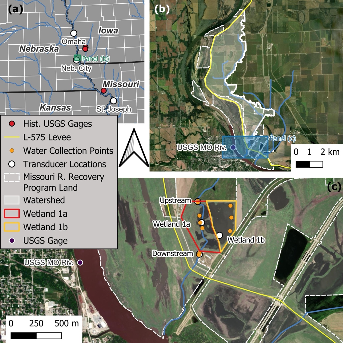
Figure 1. Map of study area showing (a) location on the border of Iowa and Nebraska (green square shows extent of panel b), (b) L-575 levee and watershed area draining to the wetland (blue rectangle shows extent of panel c), and (c) sampling points within the individual wetland cells and up and downstream, as well as the location of the USACE levee and the USGS Missouri (MO) River gage. Note the three water quality collection points in each area (orange dots) were composited in the field. Basemap is ESRI World Imagery (ESRI 2026); sources: Esri, DigitalGlobe, GeoEye, i-cubed, USDA FSA, USGS, AEX, Getmapping, Aerogrid, IGN, IGP, swisstopo, and the GIS User Community.
3. Materials and Methods
3.1. Field Data Collection
Wetland hydrology and water quality were monitored from September 2023 to November 2023 and from March 2024 to October 2024. We did not monitor during the winter because the wetlands were frozen and nutrient removal was assumed to be limited due to low biological activity. Water depths were measured every 15 minutes in the wetland and up- and downstream using Onset® HOBO U20 leveloggers installed in stilling wells, with one barologger installed along a high bank for atmospheric pressure compensation. Figure 1c shows the location of individual water sample locations in the Wetland 1a and Wetland 1b cells, and upstream and downstream. Composite water samples were collected approximately every 2 weeks at each location (Figure 1c) and sent to a private lab (Suburban Laboratories, Inc., Geneva, IL) for analysis for:
Total N (TN) and Total Kjeldahl N (TKN) (standard method 4500N[org)])
Nitrate + nitrite (standard method SM-E353.2)
Ammonium (standard method 4500NH3)
Total P (TP) and ortho-phosphate (standard method 4500P) species.
Composite samples consisted of 3, 1-L samples collected just below the water surface in each sampling zone (e.g., Wetland 1a), which were then combined. After collection, samples to be analyzed for TN, TKN, and TP were acid-preserved (H2SO4). All sample bottles were placed in a cooler and shipped to the lab within 24 hours. A Hydrolab® multiparameter sonde was used to measure dissolved oxygen (DO), specific conductance, pH, and chlorophyll concentration at each sample location.
3.2. Watershed Hydrologic Model
We used SWAT+ (Arnold et al 2025) to simulate runoff and nutrient loading from the watershed. SWAT+, an upgraded version of the Soil and Water Assessment Tool (SWAT) (SWAT 2026), is widely used for simulating surface runoff, sediment transport, and water quality, especially in agricultural watersheds (Arnold et al 2012; Bieger et al 2017). Briefly, SWAT+ divides the watershed into hydrological response units (HRUs) of relatively uniform land use, soils, and slope and simulates surface and subsurface hydrology and nutrient transport and transformation processes. The sources for model input data are shown in Table S1.
3.2.1. Model Setup
We used the QGIS SWAT+ plug-in (QSWAT+ version 3.03) (QSWATPlus 2026) to incorporate spatial information such as the stream network, management practices, weather data, soil data, and land use/cover maps into the hydrological model. The watershed was delineated using the downloaded digital elevation model (DEM), which was burned with an existing stream network shapefile. A threshold area of 0.1 km² was applied to define the channel network. HRUs were generated by incorporating land use files, soil files, and land use lookup table (Olaoye et al 2021) and soil data from SSURGO (Soil Survey Staff 2019). A filter was applied to consider only areas greater than 100 ha (Forgrave et al 2024) to reduce computational complexity.
We used the SWAT+ Editor (version 3.0.8) for editing inputs and running the model. Historical weather data including precipitation, humidity, and temperature for the nearest weather station (in Nebraska City, Nebraska, United States) were imported, while solar radiation, relative humidity, and wind speed were generated in SWAT+. The Muskingum routing method was applied for flow routing, while the Hargreaves method was used to estimate potential evapotranspiration (PET). All simulations were done using a daily time-step.
3.2.2. Model Calibration
We performed a 2-step calibration process. First, we performed hydrologic calibration to ensure the model accurately predicted watershed outflows. Next, we used this hydrologically calibrated model and further calibrated nutrient parameters to match observed nutrient loads (Figure 2). The study watershed has no observed flow data to use for calibration. We therefore found 3 nearby watersheds of similar size and land use with historic USGS stream gages to use for model calibration (data from 1953-1964). For each site, we calculated a daily flow duration curve (FDC), standardized by watershed area, and averaged values at each flow percentile. Next, this average, unit-area FDC was scaled by study watershed area to obtain a representative FDC for the watershed. We then compared this FDC with the SWAT+-modeled FDC for hydrologic calibration (after Westerberg et al 2011). Although this was an indirect calibration approach, it allowed us to confirm that SWAT+ provides a reasonable distribution of daily flows, even if we could not compare observed flows and simulated flows on any specific day. Using historic data >60 years old was also a limitation, but land use (dominated by row crop agriculture) has been relatively consistent in these watersheds.
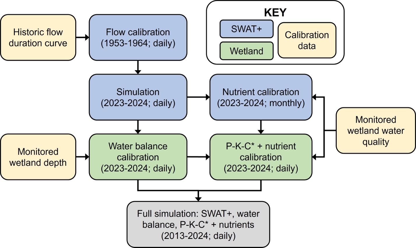
Figure 2. Conceptual scheme of the modeling approach for both the watershed and wetland.
The SWAT+ Toolbox (Chawanda 2021) was used to calibrate the modeled outflow from the watershed. First, a sensitivity analysis was conducted to evaluate the impact of various SWAT+ parameters on hydrologic variables and to identify the most significant parameters for calibration, following the Sobol method (Sobol 2001). Of the initial 19 SWAT+ parameters identified, we used only the 9 most sensitive parameters for final calibration (Table S2).
The model was calibrated for a 10-year simulation period (1955-1964), corresponding to the period for which surface flow data was available. A 2-year warm-up period (1953-54) was applied to stabilize the model before the simulation. We used 100 model iterations for calibration. The accuracy of the calibrated SWAT+ model was assessed using 3 widely used statistical parameters: Percent Bias (PBIAS), Nash–Sutcliffe Efficiency (NSE), and the Coefficient of Determination (R²) (calculated based on comparisons of modeled and “observed” FDC). If the simulated flow closely matched the observed data (e.g., high NSE and R² values, low PBIAS), it indicated that the model accurately represented the hydrological processes in the watershed (Moriasi et al 2015). Calibrated values obtained from the SWAT+ Toolbox were manually incorporated into QSWAT+ by modifying the input files. This flow-calibrated model was then used for nutrient calibration.
The flow-calibrated model setup was used to calibrate monthly TN and TP loads. Monthly observed data for TN and TP concentrations were available for the period of September 2023 to September 2024. We multiplied these concentrations by the average monthly flow rates from the calibrated SWAT+ model to get monthly nutrient loads. Using the SWAT+ Toolbox, the same calibration methodology was applied, starting with a sensitivity analysis to evaluate the impact of various SWAT+ parameters on water quality variables. Initially, 26 SWAT+ parameters were selected for optimization, all of which showed sensitivity to TN and TP (Table S3).
3.3. Wetland Modeling
3.3.1. Wetland Water Balance
A wetland water balance was constructed, where inputs included direct rainfall on the wetland surface and surface inflow, while losses occurred through evapotranspiration and surface outflow. Groundwater could be either an input or output, depending on the direction of groundwater flow. The overall water balance was represented by Eq. 1 (Kadlec and Wallace 2009; Wallace et al 2022):
Vt = Vstored + Qin + Qp ± Qg – QET – QOUT Eq. 1
where Vt represents the water storage at the end of the time step; Vstored is the water stored at the beginning of the time step; Qin and Qout denote the surface inflow and outflow of the wetland, respectively; Qp accounts for direct rainfall; Qg represents groundwater into/out of the wetland, and QET corresponds to evapotranspiration from the wetland area. Qin was modeled watershed surface runoff from SWAT+. No surface outflow was observed during the field data collection period (9/2023 – 11/2023 and 4/2024 – 10/2024). No outflow occurred because in 2023, the wetland water surface elevation was never high enough to exit the outflow culvert, and in 2024, high Missouri River water levels prevented water flow through the culvert flap gate. Qout was therefore set to zero for the baseline modeling. Direct rainfall was calculated as:
Qp = i * A Eq. 2
where i is the rainfall rate (m/day) and A is the area of the wetland (m2).
Groundwater flow between the river and the wetland (under the levee) was modeled using the Dupuit equation, assuming saturated flow in an unconfined aquifer. There is some uncertainty in the hydraulic conductivity value (K) to use, so we calibrated this value by comparing observed and modeled water levels.
The basic equation was:
\(Q_{g} = W*\frac{K}{2X}\left(h_{0}^{2}-h_{1}^{2}\right)\)Eq. 3
where the Qg (m3/day) is positive for inflow into the wetland and negative for outflow. It is influenced by the width of flow (W = 900 m, estimated based on the width of the wetland), hydraulic conductivity (K), and the levee width (X = 80 m). The water elevation on the riverward side (h0) was determined using the river water level (USGS gage 06807000, Figure 1b, Figure 1c), while the water elevation on the wetland side (h1) was calculated based on modeled wetland water elevations. Modeled wetland water elevations were used as these were dependent on all modeled components of the water balance. These modeled values were compared to observed water elevations to calibrate K. Both river and wetland water elevations were based on an assumed aquifer bottom of 261 m above sea level. This was selected as a reasonable value for aquifer thickness. Adjusting this value would have resulted in a different calibrated K value, but would not have changed the modeled groundwater fluxes.
Potential evapotranspiration (PET) was estimated by the Hargreaves method (m/day), and the wetland area (A), following (Lyu et al 2024).
QET = PET * A Eq. 4
Water depth in the wetland was calculated based on stored volume and a depth-area-volume relationship developed in QGIS using a DEM of the wetland. We simulated wetland water balance dynamics annually from April to December, omitting the winter months when ice and snow accumulation are influential, but for which we had no observational data. Each year, we assumed an initial water depth of 6.0 cm. This assumed minimal carry-over of stored water from the previous year and was based on field observations during the monitoring period.
3.3.2. Wetland Nutrient Mass Balance
The nutrient mass balance in the wetland is presented in Eq. 5:
Mt = Mo + Min + Md + Mg – Mr Eq. 5
where Mt is the nutrient mass (kg) at the end of the time step (1 day) and Mo is the initial nutrient mass (kg) at the beginning of the time step. Min represents the nutrient input from surface inflow (kg), while Md accounts for atmospheric deposition (kg) from direct rainfall input. The rainfall contribution was estimated using an average TN concentration of 500 μg/L (Wallace et al 2022). This is the median of values reported for sites in the U.S., with a range of 300 μg/L –1,900 μg/L (Eriksson 1952). Atmospheric deposition was a relatively small input (~3% of the total N mass balance) and changing the rainfall concentration would likely have had only a minor effect on the results. P atmospheric deposition was considered negligible. Mg represents nutrient exchange with groundwater (kg), influenced by river nutrient concentrations (TN and TP), with data provided from long-term USACE monitoring on the Missouri River at Nebraska City (Brent Dinkel, USACE). Mg was calculated as follows:
Mg = (TN or TP concentration) * Qg Eq. 6
If the Qg originated from the river, the TN and TP concentrations of the river were used. We multiplied these values by 0.5, assuming 50% of this nutrient load was attenuated as it flowed through the aquifer. The amount of nutrient attenuation in alluvial aquifers can vary widely depending on flow path length/time, redox conditions, and soil type (Lewandowski and Nützmann 2010). In general, nitrate-nitrogen is removed primarily via denitrification, while P is removed through absorption (although P can also be released from soils under reducing conditions) (Hoffmann et al 2006). We assumed 50% nutrient load attenuation to account for these processes in lieu of site-specific data, recognizing that this would introduce error into our analysis. Conversely, if the Qg was leaving the wetland, the TN/TP concentrations of the wetland were used in Eq. 6.
Mr denotes nutrient removal within the wetland (kg) through mechanisms such as plant uptake, denitrification, absorption, and sedimentation. We tested both the K-C* and P-K-C* models and the difference was not significant. Therefore, we proceeded with the P-K-C* model to simulate the combined effects of all removal processes:
\(\frac{(C_{\text{out}} - C^*)}{(C_{\text{in}} - C^*)} = \left(1 + \frac{K_t\tau}{\mathrm{Ph}}\right)^{-P}\)Eq. 7
where P = number of cells in series, dimensionless (4 for TN and TP) (Kadlec and Wallace, 2009); τ is the detention time (1 day for a daily calculation time step); and h is the water depth (m). C* is the background nutrient concentration and was estimated as 0.65 mg/L for TN and 0.04 mg/L for TP based on the lowest observed concentrations in the wetland. Kt is the first-order areal rate coefficient (m/day) that can be calculated as follows:
Kt = K20 * θ(T-20) Eq. 8
where θ is the modified Arrhenius temperature factor (dimensionless) and K20 is the rate constant at 20 °C, and T represents water temperature (°C). We calibrated both θ and K20 based on observed nutrient concentration data. The mass of nutrient removal was calculated as:
Mr = (Cin – Cout) * Vstored Eq. 9
where Cin is the concentration of TN/TP (mg/L) at the beginning of the time step and Cout is the concentration of TN/TP (mg/L) at the end of the time step. All wetland water and nutrient mass balance modeling was performed treating Wetland 1a and Wetland 1b as a single wetland unit.
3.4. Wetland Model Scenarios
The fully calibrated SWAT+ and wetland water and nutrient balance models were used to assess wetland nutrient removal performance from 2013 – 2024 (April – December), examining how inter-annual climate variability impacts wetland performance. In addition to this baseline scenario, we ran additional simulations with variable watershed or wetland characteristics. The goal of these simulations was to determine how nutrient removal performance was affected by changing nutrient loads and modifying wetland design.
3.4.1. Increasing Nutrient Loading
Initial results suggested that the wetland could adequately retain watershed nutrient inflows. We tested the resilience of this nutrient removal performance by artificially increasing nutrient inflow loads. We simulated nutrient inflows at loads 2, 5, and 10 times higher than those modeled from SWAT+. The wetland nutrient mass balance was re-calculated with these modified nutrient inputs.
3.4.2. Passive Depth Control
A culvert allows outflow from the wetland to pass through the levee and drain to the Missouri River. However, culvert design and high river water levels (like was experienced for much of the field observation period in 2024) prevent wetland drainage, and therefore no culvert outflow was modeled for the baseline scenario. To test the effects of different culvert configurations, we simulated a variety of scenarios with a 0.3048-m (1-ft) diameter culvert, 0 cm, 30 cm, and 60 cm above the wetland bottom. The difference in elevation between the river and the wetland was used to calculate the potential volume of water discharged from the wetland, and to determine whether the wetland could drain (i.e., only when wetland water elevation was greater than river water elevation). This discharged volume was then subtracted from the water balance equation (Eq. 1).
The daily discharge volume was determined by the culvert’s discharge capacity, which governs the water flow from the wetland to the river. This capacity can be calculated using the equation for flow through an orifice, under the assumption that the submerged inlet functions similarly to an orifice flow device:
\(Q_{\text{out}} = C_d * A * \sqrt{2gh} * 86400\)Eq. 10
where Qout = flow rate (m³/day), Cd = discharge coefficient (dimensionless, assumed 0.67), A = area of the submerged inlet (m²), g = gravitational acceleration (9.81 m/s²), and h = head difference (m), or the depth of water above the culvert opening. The mass of nutrients leaving the wetland (kg/day) was calculated as follows:
Mout = Qout * Cout * 10-3 Eq. 11
where Cout represents the concentration of TN/TP at the end of each time step (mg/L). This value was then incorporated into the nutrient mass balance equation as follows:
Mt = Mo + Min + Md + Mg – Mr – Mout Eq. 12
3.4.3. Wetland Size
Wetland size plays a crucial role in both water balance and nutrient mass balance. To assess the impact of size variation, 2 alternative wetland areas, representing 50% (10.5 ha) and 150% (31.5 ha) of the current wetland, were evaluated. This analysis aimed to establish thresholds for how changes in wetland size influence nutrient removal capacity under consistent operational conditions.
4. Results and Discussion
4.1. Field Data Results
Nutrient concentrations varied over the monitoring period (Table S4, Figure 3). TN and TP concentrations generally peaked at all locations in March 2024, followed by a gradual decline throughout the rest of the year. This initial spike likely reflected nutrient accumulation during winter and low initial water depth in spring, prior to the onset of surface runoff and active wetland treatment. The subsequent reduction in nutrient levels was associated with rising temperatures and increased pH and DO levels (Table S4), indicating enhanced biological activity and treatment efficiency. Nutrient concentrations were generally highest upstream, and lowest in Wetland 1a. Concentrations in Wetland 1b were generally higher than in Wetland 1a (especially for N), potentially because Wetland 1a is shallower and more vegetated, which could have increased nutrient removal. Most N was organic (high Total Kjeldahl N, low NH4+ and NO3+NO2; Table S4), but there was a substantial inorganic P fraction for most of the sampling period. Missouri River concentrations of both TN (median = 2.55 mg/L, range = 0.32 mg/L – 8.92 mg/L) and TP (median = 0.21 mg/L, range = 0.04 mg/L – 2.9 mg/L) were slightly higher on average compared to nutrient concentrations in the wetland. Monitored wetland depth showed strong influence of Missouri River water levels (via groundwater exchange), especially during 2024 (Figure S1).
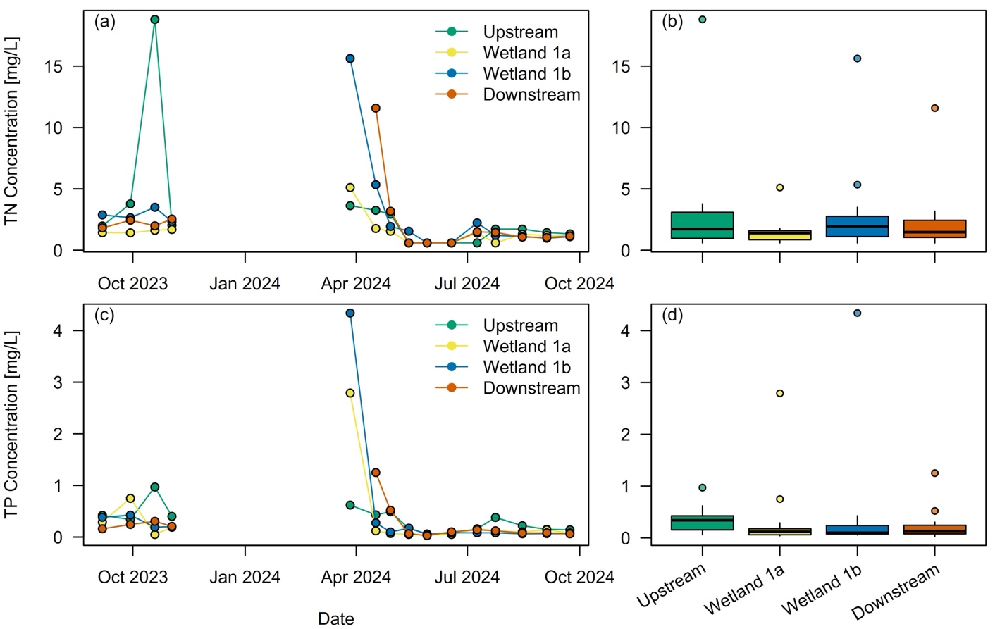
Figure 3. Monitoring data showing TN and TP concentrations over time (a and c) and boxplots of concentrations by location (b and d). Values below the reporting limit were set to half this value.
4.2. SWAT+ Calibration
The calibrated SWAT+ model demonstrated good performance in simulating daily flow rates in the watershed (Figure S2). High NSE (0.84) and R² (0.98) values indicated good agreement with the observed flow duration curve. Simulations generally underpredicted flow rate (PBIAS = -24.2%), but total runoff volume error was low (2.2%). Overall, these results suggested that SWAT+ effectively captures the magnitude, frequency, and variability of watershed flow. SWAT+ calibration for monthly nutrient loads showed generally lower accuracy (R2 and NSE values of ~0.6; Figure S3). However, SWAT+ was able to predict temporal trends in loads relatively well.
4.3. Wetland Model
4.3.1. Wetland Model Calibration
The wetland water balance was calibrated by comparing observed and modeled wetland depths, giving a calibrated K value of 14 m/day (1.6 x 10⁻⁴ m/s). This value is relatively high but not unreasonable for the sandy soils present in this area. It is within the range of other estimates of hydraulic conductivity in Missouri River floodplains (0.02 m/day – 38 m/day, Buchmiller 1988; and 0.9 m/day – 87 m/day, Hassler 2005). Overall, the simulated depths agreed reasonably well with the observations (R2 = 0.96, NSE = 0.86), although the model slightly overestimated water depth during the summer of 2024 (PBIAS = 17.7%) (Figure S4). This could indicate our calibrated K value was too high, but lowering K resulted in inaccurate modeled water levels in fall 2023.
We calibrated the rate constant of the P-K-C* model using water quality observations and the wetland nutrient mass balance (Eq. 5). Calibrated values of K20 were 5.0 m/yr and 10.0 m/yr for TN and TP, respectively. Calibrated θ values were 1.17 for both TN and TP. The R² values were 0.88 for TN and 0.96 for TP, indicating good agreement between modeled and observed data (Figure S5). The calibrated K20 value for TN is near the 20th percentile of literature values and equal to the median value for TP (Kadlec and Wallace 2009), suggesting relatively conservative N removal but typical P removal rates compared to other wetland systems. We used constant K20 values over the whole modeled period. This neglects potential changes in nutrient removal rates as the wetland ages (Mitsch et al 2014).
4.3.2. Baseline Scenario – Water Balance
Figure 4 presents the modeled wetland water balance for 2013 to 2024, showing both water depth and annual contributions of different water balance components. Annual patterns are similar to observed depths for 2023 to 2024, with a peak in the summer and decrease into the fall. However, the magnitude of fluctuations is highly variable year-to-year, driven primarily by differences in rainfall (changing surface inflows) and Missouri River water levels, which control the magnitude (and direction) of groundwater fluxes. For example, the Missouri River flooded for much of 2018 and 2019, as evidenced by persistent high-water levels in the wetland. Contributions from different sources significantly influenced wetland hydrology over time (Figure 4b). Surface inflow was the primary contributor to water inputs, with groundwater outflow or ET being the largest water loss, depending on the year (Table S5). Surface inflow was high from 2014 to 2019, but it was much lower from 2020 to 2024 due to lower annual precipitation. Groundwater outflow generally exceeded groundwater inflow, except for 2018 to 2019. Higher river levels during those years prevented the wetland from draining via groundwater outflow, resulting in high wetland water depths at the end of the year.
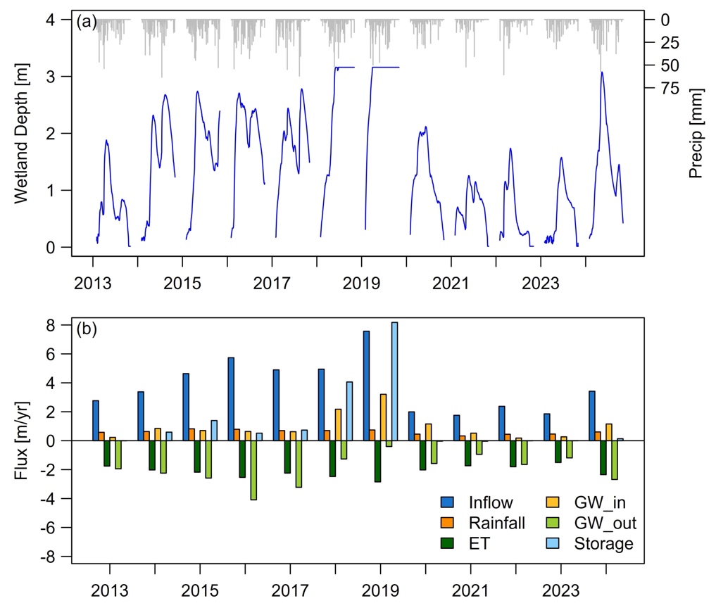
Figure 4. Changes in water balance components in the wetland from 2013 to 2024: (a) variation in water depth and precipitation over time; (b) annual water balance values represented in m/yr. Note storage is the increase (+) or decrease (-) in total water volume in the wetland from the beginning to the end of the year. ET = evapotranspiration, GW_in = groundwater in, GW_out = groundwater out.
4.3.3. Baseline Scenario – Nutrient Mass Balance
Modeled wetland TN concentrations showed consistent annual patterns, beginning high in April and decreasing through the year (Figure 5a). Concentrations were relatively stable from July to December. Surface inflow was relatively low beginning in early summer. Additionally, higher water temperatures during the summer increased N removal, resulting in concentrations declining to near background, where they remained through the fall. Annual variability in concentration patterns can also be seen, with peaks in concentration largely driven by runoff events delivering N loads from the watershed.
Surface runoff was the dominant inflow source for half of the years, while groundwater inflow was the primary contributor for the other years (Figure 5b). Groundwater outflow accounted for the largest mass loss in most years except for 2018 to 2021, when removal was larger. High amounts of N remained stored in the wetland at the end of both 2018 and 2019, when high Missouri River levels prevented wetland drainage. The average removal rate over the modeled period was 10.4±6.2 kg N ha-1 yr-1, substantially lower than reported by Mitsch et al 2000 (100 kg N ha-1 yr-1 – 400 kg N ha-1 yr-1 for wetlands treating agricultural and urban runoff in the eastern U.S.). The comparatively lower removal loads observed in our system were likely due to relatively low inflowing N loads (average total input of 32.2 kg N ha-1 yr-1), which left less N to be removed (Table 1).
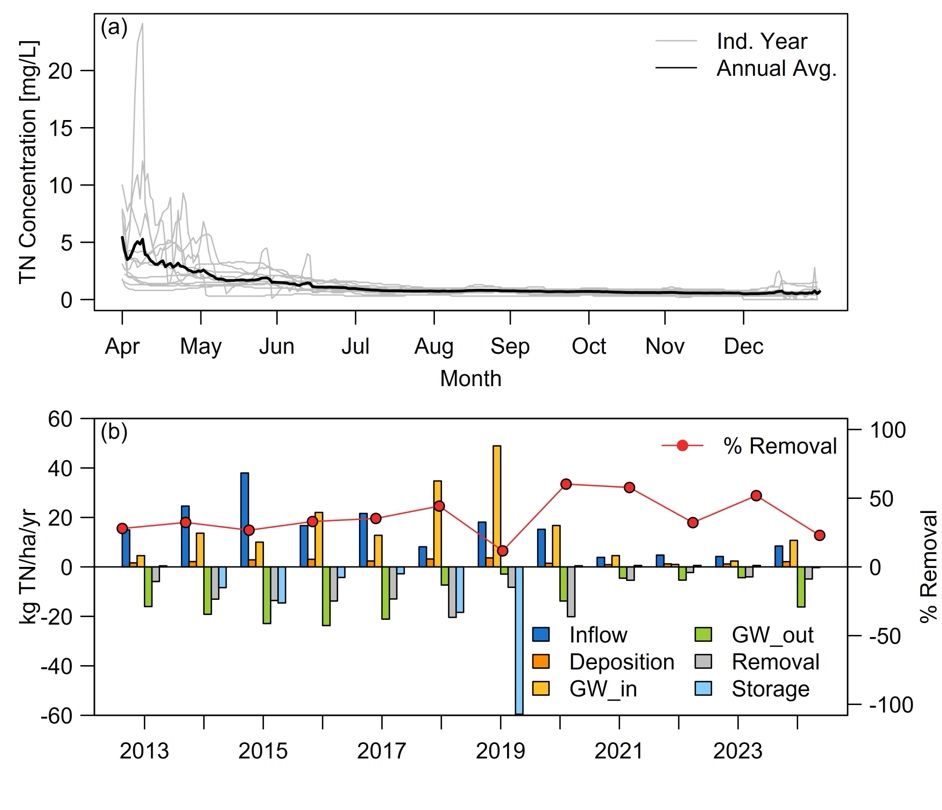
Figure 5. (a) Modeled TN concentrations in the wetland from 2013 to 2024, showing results from individual years and an average across all years; (b) TN mass balance from 2013 to 2024, including annual percent removal rate. Note that storage is the mass of TN remaining in the wetland at the end of each simulation year. GW_in = groundwater in, GW_out = groundwater out.
TN removal efficiency averaged 36.4±14.5%. However, significant year-to-year variability was observed, with an especially low removal rate in 2019 (11.7%). Removal efficiency tended to be higher and mass removal rates lower in years with lower incoming loads and hydraulic loading rates. The average of 36.4% TN removal was largely in line with previous studies (Table 1), although there is high variability reported in the literature. Our modeled TN removal rates and efficiencies may have been lower than others due to the large fraction of organic N in our system, which is not as easily removed as more reactive forms of N (Kadlec and Wallace 2009). Furthermore, our monitoring data showed inflowing N concentrations near background for much of the year (following a spring peak), which limits N removal potential.
Annual TP concentrations showed similar patterns to TN, with a spring peak followed by a gradual decline (Figure 6a). Surface runoff was the dominant source of TP throughout the study period, although groundwater inflow was substantial in years with higher river levels (Figure 6b). Groundwater outflow was highly variable, and like groundwater inflow, was influenced primarily by river levels. These results highlight the crucial role of hydrological conditions, especially flood events, in shaping P loading and retention dynamics. TP removal rates were higher than for TN, but showed similar annual trends (e.g., lowest in 2019). Also, like TN, TP percent removal rates were higher but mass removal rates were lower in years with lower incoming loads. The average TP removal efficiency (62.6%±16.9%) was on the high end of those reported in the literature (Table 1). Like N, TP loading rates (5.7±2.9 kg P ha-1 yr-1) were on the lower end of literature values (Table 1). For example, we were within the range reported in a comprehensive literature review (0.3 kg P ha-1 yr-1 – 3,730 kg P ha-1 yr-1), but well below the median (32 kg P ha-1 yr-1) (Land et al 2016).
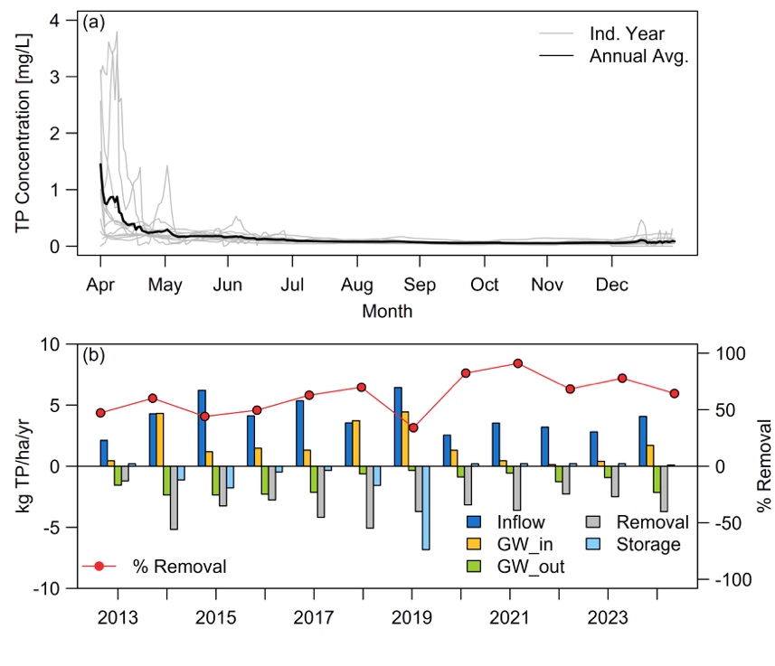
Figure 6. (a) Modeled TP concentrations in the wetland from 2013 to 2024, showing results from individual years and an average across all years; (b) TP mass balance from 2013 to 2024, including annual percent removal rate. Note that storage is the mass of TP remaining in the wetland at the end of each simulation year. GW_in = groundwater in, GW_out = groundwater out.
4.4. Scenario Modeling
4.4.1. Increasing Nutrient Loading
Increased surface nutrient loading (2x, 5x, and 10x the baseline) led to substantially higher nutrient concentrations, especially early in the year (April – July, Figure S6). Increasing surface loading 10x led to a roughly 6-fold increase in peak TN and TP concentrations; however, this difference substantially diminished by the fall. Notably, nutrient concentrations remained higher under the elevated inflow scenarios compared to the baseline. These patterns indicate that extreme nutrient loading can temporarily exceed the wetland’s treatment capacity. Nevertheless, the system exhibited resilience and recovery over the year, as lower surface inflows during the summer and fall allowed for accumulated nutrients to be removed. The minor rise in nutrient concentrations during December was likely due to lower temperatures reducing removal, as well as shallower water in the wetland, meaning relatively small changes in nutrient mass can result in large changes in concentrations.
Increases in upstream nutrient loading led to increases in removal, export via groundwater, and nutrient storage at the end of the year (Figure 7a and Figure 7b, Table S6). Under the most extreme, 10x loading increase, absolute removal rates increased over 7x (10.4 kg N ha-1 yr-1 to 75 kg N ha-1 yr-1 and 3.4 kg N ha-1 yr-1 to 26 kg P ha-1 yr-1). Removal efficiency also increased for TN (improving from 36.4% to 50.0%), with much smaller changes for TP (increasing from 62.6% to 65.2%). Surface loading increases for both TN and TP increased by the same factor, but total loading for TN (surface runoff + deposition + groundwater inflow) increased less than for TP (surface runoff + groundwater inflow), explaining the difference in increase removal efficiency. Even for the most extreme scenario (10x loading), total N and P loading rates to our wetland were similar to or lower than what has been reported for other wetlands (Table 1), suggesting this scenario is realistic for agricultural systems.
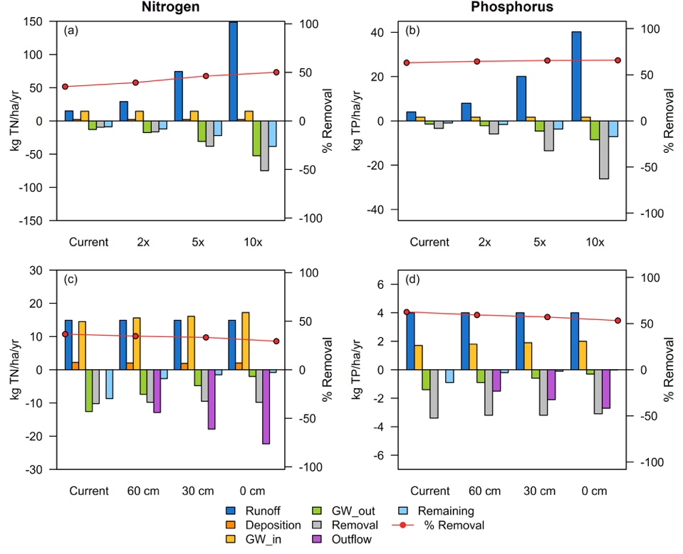
Figure 7. Effects of various levels of increased upstream nutrient loads (a and b) and installation of drainage culvert (c and d) at different elevations on N and P mass balance and percent removal rates. GW_in = groundwater in, GW_out = groundwater out.
Overall, these results indicated that the wetland had sufficient capacity to remove even much higher loadings of TN and TP than it currently experienced. This consistent performance suggests a high level of functional resilience, with the system capable of absorbing substantial external pressures without a proportional decline in treatment efficiency. This appears to be especially true for N (which saw increases in removal efficiency), while P removal efficiency may be near its maximum (although mass removal rates still increase). This analysis assumes that removal rate constants (K20) remain the same and that incoming nutrient loads increase, but hydraulic loading rate does not. This also explains the opposite behavior seen in the baseline modeling (Figure 5 and Figure 6) where higher removal efficiencies were observed in years with lower incoming loads. These years also had low hydraulic loading rates, which allowed for more efficient nutrient removal. Others have shown that removal efficiencies increase with increased loading, especially if hydraulic loading rates remain the same (Land et al 2016; Ross and McKenna 2022). This suggests that removal efficiency in the study wetland was primarily limited by hydraulic loading rate, rather than incoming nutrient loads.
4.4.2. Passive Depth Control
We modeled the effect of a culvert set at different elevations (0 cm, 30 cm, and 60 cm) on the water and nutrient mass balance in the wetland. Simulated water depth followed a consistent pattern, with little difference in depth with and without the culvert through spring and early summer (when high Missouri River water levels restrict culvert outflow), followed by faster draining of the wetland when the culvert was in place (Figure S7a). Outflow from the culvert decreased both groundwater outflow from the wetland and the amount of stored water at the end of each year (Figure S7b). This suggests that the culvert increased both the total outflow from the wetland and impacted how the water left the wetland (surface vs subsurface flow), which had implications for nutrient export.
The incorporation of the culvert did not substantially alter TN/TP concentrations overall, but it did impact the TN/TP loads (Figure 7c and Figure 7d, Figure S8, Table S7). Similar to the water balance, adding a culvert increased the mass of TN and TP exported via surface outflow while simultaneously decreasing groundwater outflow and nutrient mass stored in the wetland at the end of the year. There was also a slight reduction in nutrient removal, resulting in lower percent removal (29.4% – 34.6% for TN, 53.3% – 59.3% for TP). These results suggest that the culvert largely replaced the natural groundwater exfiltration pathway, enhancing drainage and allowing for more depth control. Generally, shallower depths increase nutrient removal and uptake by enhancing oxygen availability, plant–water interactions, and biogeochemical exchanges at the sediment surface (Kadlec and Wallace 2009; Alahmady et al 2013; Carpenter and Bledsoe 2025). However, this benefit for nutrient removal seemed to be counterbalanced by increased wetland drainage and, therefore, lower retention times when the culvert was in place. The 60 cm culvert had water and nutrient mass balances most similar to the baseline, no-culvert scenario, suggesting passive depth control can help maintain shallower depths while only minimally impairing nutrient removal. A particular challenge in this wetland was that depth control is very limited when Missouri River water levels are high, preventing any surface outflow from the wetland. Other riverine CWs may be similarly influenced by river hydrology (or be inundated during floods); however, riverine wetlands in the literature tend to receive pumped or controlled river water and may be less hydrologically connected to the adjacent river (Jia et al 2014; Mitsch et al 2014).
4.4.3. Wetland Size
Reducing the wetland area to 50% of its original size (to 10.5 ha) while maintaining constant inflow volume resulted in a substantial increase in average hydraulic loading rate (5.3 m/yr to 9.3 m/yr) (Figure S9). This increase in hydraulic loading reduced nutrient removal efficiency (36.4% – 23.4% for TN and 62.6% – 47.7% for TP; Table 2) but slightly increased TP mass removal rates (Table 2, Figure S10; TN mass removal is unchanged). Increasing wetland area by 50% (to 31.5 ha) slightly reduced hydraulic loading (5.3 m/yr to 4.0 m/yr) and increased removal efficiency (36.4% to 46.8% for TN and 62.6% to 70.5% for TP; Table 2). These results reinforce that nutrient removal performance in this wetland is more sensitive to HLR than to nutrient loading, and that increasing wetland size can increase removal (although potentially at much higher expense). Smaller wetland areas under constant loading are more prone to hydraulic overloading, which shortens residence times and diminishes the conditions necessary for effective biological uptake and microbial transformation of nutrients. The current wetland size (~1.3% wetland:watershed area ratio) is on the lower end of the recommended/typical range of agricultural CWs (e.g., Carpenter and Bledsoe 2025, Gaballah and Lammers 2025).
While our analysis suggests the wetland can adsorb higher nutrient loads, this area adjustment analysis shows that hydraulic loading rate may be the limiting factor in wetland performance. Removal efficiency generally declines with increased hydraulic loading rate (Crumpton et al 2020). We observed relatively large declines in performance for our smaller wetland, even if the hydraulic loading rate (9.3 m/yr average) was lower than many similar wetlands (Table 1; Gaballah and Lammers 2025). Additional scenarios explored the interaction between wetland size, nutrient loading increases, and passive depth control. The outcomes were variable (Table 2), but generally showed that, all else being equal, nutrient removal efficiency was most affected by wetland size, followed by increasing upstream nutrient loads and finally, passive depth control.
Table 1. Nutrient retention in created and natural wetlands receiving inflows of nutrients from river overflows and agricultural runoff compared with the current study. HLR = hydraulic loading rate.
| Wetland Location | Wetland Area (ha) | HLR (m/yr) | TN Loads (kg N ha−1 yr−1) |
TN Removal (%) | TP Loads (kg P ha−1 yr−1) |
TP Removal (%) | Reference |
| Iowa (26 wetlands) | 300 total | - | 157- 16,800 (avg. 6,750) | 35 | - | - | Crumpton et al (2020) |
| Wilma H. Schiermeier Olentangy River Wetland Research Park, OH |
2 | 39.8 | 1220 | 31.8 | 56.1 | 42.8 | Mitsch et al (2014) |
| Wilma H. Schiermeier Olentangy River Wetland Research Park, OH |
3 | 20±4 | 645.0 | 41.0 | 61.0 | 31.0 | Fink and Mitsch (2007) |
| Everglades Nutrient Removal Project, Florida | 1545 | - | 315.6 | 55.0 | 11.7 | 82.0 | Moustafa (1999) |
| Ohio River basin, Ohio | 1.2 | 6.5 | - | - | 71.0 | 51.2 | Fink and Mitsch (2004) |
| Yakima Basin, Washington |
1.6 | - | - | - | 40-100 | 37-43 | Beutel et al (2014) |
| Breton Sound Estuary, Louisiana Delta | 110,000 | - | 35.0 | 86.0 | - | - | Lundberg et al (2014) |
| Timberlake Restoration Project, North Carolina | 440 | 8.95 | 9.95 | - | 0.3 | 14-50 | Ardon et al (2010) |
| 112-146 wetlands worldwide | 0.00001-1,000 | - | 21.2-24,860 | -12.8-93 | 0.3-3,730 | -422-99 | Land et al (2016) |
| 19 wetlands treating agricultural runoff | 0.1-1087 | - | - | - | 0.3-2,000 | 7-60 | Skinner (2022) |
| Agricultural wetlands, IL | 0.3-0.8 | - | 552.2-885.8 | 31.3-43 | 6.67-9.2 | 27.8-43.7 | Kovacic et al (2000) |
| Lake Apopka, Florida | 308 | 32-49 | - | - | 50-60 | 30.0 | Dunne et al (2012) |
| Lake Apopka, Florida | 276 | 44-112 | - | - | 32.4 | 26.2 | Dunne et al (2015) |
| Mackay, north Queensland, Australia | 2.5 | - | 226.3 | 36.7 | - | - | Wallace et al (2022) |
| Fremont County, IA | 21.0 | 5.31 | 32.2±24.5 | 36.4±14.5 | 5.7±2.9 | 62.6±16.9 | This study |
Collectively, these scenarios suggest that a design approach that prioritizes sufficient surface-area to watershed-size ratio and incorporates understanding of total nutrient loading (both surface and subsurface) will likely be most successful for optimizing nutrient removal. For example, we showed that increasing wetland size by 50% decreased HLR and depth and increased nutrient removal efficiency. While per area mass removal rates (kg TP or TP ha-1 yr-1) were slightly smaller in the larger wetland (Table 2), the total mass removal was highest for this scenario due to larger wetland area. On the other hand, smaller wetlands had higher per area mass removal rates, showing that these smaller wetlands can be effective in areas where land availability is constrained. Our model scenarios also showed that depth control can be used to provide more depth stability, which may slightly decrease nutrient removal but could provide additional ecological benefits, such as increasing vegetation and waterfowl species diversity (e.g., Carpenter and Bledsoe 2025). However, depth control was highly constrained by the hydrologic influence of rivers adjacent to these borrow pit wetlands. Design of floodplain wetlands should incorporate riverine hydrologic connectivity (both surface and subsurface) when calculating hydraulic and nutrient loading rates. Furthermore, designers should determine the timing and duration of high river levels that may limit outflow from the wetland and substantially increase wetland depth. If these are determined to significantly impair wetland function, alternative outlet designs or pumping systems may need to be considered.
Table 2. Comparison of wetland performance under different modeled design scenarios and modifications. Percent removal for each scenario is shown with mass removal rates (kg TN or TP/ha/yr) in parentheses.
| Nutrient | Scenario | Current | Area Size | ||
| 150% | 50% | ||||
| TN | Current | 36.4% (10.4) | 46.8% (10.2) | 23.4% (10.4) | |
| Increasing loading inflow | 2x | 40.1% (17.3) | 50.2% (15.6) | 26.5% (19.7) | |
| 5x | 46.5% (38.8) | 55.8% (32.1) | 31.9% (50.0) | ||
| 10x | 50.0% (75.0) | 58.9% (59.8) | 34.8% (101.3) | ||
| Adding culvert (elevation) | 0 cm | 29.4% (9.1) | 35.7% (8.3) | 19.8% (9.8) | |
| 30 cm | 33.3% (9.5) | 43.3% (9.7) | 22.3% (10.4) | ||
| 60 cm | 34.6% (9.8) | 45.1% (9.8) | 22.9% (10.7) | ||
| TP | Current | 62.6% (3.4) | 70.5% (2.8) | 47.7% (4.5) | |
| Increasing loading inflow | 2x | 63.9% (5.9) | 71.2% (4.6) | 49.2% (8.5) | |
| 5x | 64.9% (13.4) | 71.6% (10.1) | 50.4% (20.2) | ||
| 10x | 65.2% (26.0) | 71.7% (19.2) | 50.8% (39.8) | ||
| Adding culvert (elevation) | 0 cm | 53.3% (3.1) | 61.7% (2.6) | 40.7% (4.2) | |
| 30 cm | 57.1% (3.2) | 66.0% (2.6) | 43.8% (4.4) | ||
| 60 cm | 59.3% (3.2) | 68.1% (2.7) | 45.6% (4.5) | ||
5. Conclusion
CWs created from borrow pits originally excavated for levee repair or setbacks offer valuable opportunities to intercept agricultural runoff before it reaches major waterways. This study demonstrated that such wetlands can function as effective treatment systems, particularly when designed and managed strategically. Monitoring and modeling show the important role played by variable Missouri River water levels in controlling groundwater dynamics (both direction and magnitude of groundwater fluxes) and surface outflow from the wetland. We found that nutrient loading to the wetland is lower than for similar systems, but that nutrient removal efficiency stayed the same or improved if loading rates were increased. Design modifications illustrated potential tradeoffs of installing outflow structures or changing wetland size. For example, a larger wetland had greater total nutrient removal, but smaller wetlands had higher per-area rates, potentially indicating higher cost-effectiveness.
Our analyses were limited by having only a single year of monitoring data and several modeling assumptions (e.g., nutrient attenuation in inflowing groundwater). Additional work should monitor other floodplain wetlands with different degrees of hydraulic conductivity, including wetlands that may be inundated periodically during floods. Furthermore, monitoring groundwater hydraulics and water quality is recommended to better determine subsurface connectivity and potential nutrient transformation. Future modeling work should also use uncertainty analysis to quantify how assumptions and uncertainty in calibrated parameters influence results.
Estimates suggest there are over 200,000 km of levees in the U.S. (Knox et al 2022), with much of this total length in agricultural areas. Ongoing efforts to set back levees to reduce flood risk (Chambers et al 2023, Serra-Llobet et al 2022) have some potential to increase nutrient retention on reconnected floodplains, but this potential is limited to times when floodplains are inundated (Jacobson et al 2022). Borrow pit wetlands, however, can supplement these efforts by intercepting agricultural runoff more or less continuously. Given the widespread use of borrow pits during levee repair and setback construction (approximately 100 acres of borrow pits created for every mile of levee realignment, USACE personal communication), there is huge potential for borrow pits to be converted to wetlands (with relatively minimal investment) to manage nutrient pollution and improve water quality.
Supplementary Material
The online version of this article contains a link to supplementary material that includes: Figure S1, Observed water depths in study wetland; Figure S2, Observed vs calibrated flow duration curve; Figure S3, Observed vs calibrated nutrient loads; Figure S4, Observed vs calibrated wetland water depth; Figure S5, Observed vs calibrated wetland nutrient concentrations; Figure S6, Average modeled nutrient concentrations for loading scenarios; Figure S7, Modeled wetland depths and water balance for culvert scenarios; Figure S8, Modeled wetland nutrient concentrations for culvert scenarios; Figure S9, Modeled wetland water balance for wetland area scenarios; Figure S10, Modeled wetland nutrient mass balance for wetland area scenarios; Table S1, SWAT+ input data sources; Table S2, Calibrated SWAT+ hydrologic parameters; Table S3, Calibrated SWAT+ nutrient parameters; Table S4, Measured wetland water quality data; Table S5, Baseline modeled water balance components; Table S6, Nutrient mass balance for loading scenarios; Table S7, Nutrient mass balance for culvert scenarios.
Acknowledgments
We are grateful to Brent Dinkel for providing field equipment and support, assistance with sample collection, and sharing Missouri River water quality data. We also wish to acknowledge Laura Knapp-Leiferman for providing field equipment and support, Aidan Coen and Lauren Uhlig for assistance with sample collection, Jenifer Netchaev and Michelle Bourne for assistance with lab contracting, and Jeff King and Burton Suedel for funding and support through the USACE’s Engineering With Nature Program. This paper is contribution #220 of the Central Michigan University Institute for Great Lakes Research. This work was supported by the U.S. Army Corps of Engineers Engineering with Nature Initiative through Cooperative Ecosystem Studies Unit Agreement W912HZ-20-2-0031.
Author Contributions Statement
Conceptualization: RL, MC, DC; data analysis: MG, RL; data curation: MG, RL; formal analysis: MG, RL; funding acquisition: RL, DC; investigation: MG, DC, SC, MC, RL; methodology: MG, DC, MC, RL; project administration: DC, MC, RL; resources: DC, RL; software: MG, RL; supervision: RL; visualization: MG, RL; writing–original draft: MG, RL; writing–review & editing: MG, DC, SC, MC, RL. All authors have read and agreed to the published version of the manuscript.
Conflict of Interest Statement
The authors have no conflict of interest to report.
Data Availability Statement
Collected water quality data and wetland depth data are available from the Zenodo public data repository: https://doi.org/10.5281/zenodo.20214472.
Related Publication Statement
Preliminary findings from this work have been presented at several academic conferences: American Ecological Engineering Society (AEES) (May 2025), International Symposium on Biogeochemistry of Wetlands and Aquatic Systems (June 2025), and Environmental and Water Resources Institute Congress (May 2024).
References
Alahmady KK, Stevens K, Atkinson S. 2013. Effects of hydraulic detention time, water depth, and duration of operation on nitrogen and phosphorus removal in a flow-through duckweed bioremediation system. J Environ Eng. 139:160–166. https://doi.org/10.1061/(ASCE)EE.1943-7870.0000627
Ardon M, Morse JL, Doyle MW, Bernhardt ES. 2010. The water quality consequences of restoring wetland hydrology to a large agricultural watershed in the southeastern coastal plain. Ecosystems. 13:1060–1078. https://doi.org/10.1007/s10021-010-9374-x
Arnold JG et al. 2012. SWAT: Model use, calibration, and validation. Transactions ASABE. 55(4):1491–1508. https://doi.org/10.13031/2013.42256
Arnold JG et al. 2025. Soil and Water Assessment Tool Plus (SWAT+) (Version 61.0.2.11) [Computer software]. Zenodo. https://doi.org/10.5281/zenodo.15114317
Beutel MW, Morgan MR, Erlenmeyer JJ, Brouillard ES. 2014. Phosphorus removal in a surface-flow constructed wetland treating agricultural runoff. J Environ Qual. 43:1071–1080. https://doi.org/10.2134/jeq2013.11.0463
Bieger K et al. 2017. Introduction to SWAT+, a completely restructured version of the Soil and Water Assessment Tool. J Am Water Resour Assoc. 53(1):115–130. https://doi.org/10.1111/1752-1688.12482
Buchmiller RC. 1988. A strategy for collecting ground-water data and developing a ground-water model of the Missouri River alluvial aquifer, Woodbury and Monona counties, Iowa. U.S. Geological Survey Open-File Report 87–452. https://pubs.usgs.gov/of/1987/0452/report.pdf
Carpenter M, Bledsoe B. 2025. Multi-objective wetland design for water quality and waterfowl habitat. J Ecol Eng Des. https://doi.org/10.70793/jeed.15
Chambers ML, van Rees CB, Bledsoe BP, Crane D, Ferreira S, Hall DM, Lammers RW, Landry CE, Nelson DR, Shudtz M, Suedel BC. 2023. Nature-based solutions for leveed river corridors. Anthropocene. 44:100417. https://doi.org/10.1016/j.ancene.2023.100417
Chawanda CJ. 2021. SWAT+Toolbox: User Manual. https://www.openwater.network/assets/downloads/SWATplusToolboxUserMannual.pdf
Crumpton WG, Stenback GA, Fisher SW, Stenback JZ, Green DIS. 2020. Water quality performance of wetlands receiving nonpoint-source nitrogen loads: Nitrate and total nitrogen removal efficiency and controlling factors. J Environ Qual. 49(3):735–744. https://doi.org/10.1002/jeq2.20061
Dunne EJ et al. 2015. Phosphorus removal performance of a large-scale constructed treatment wetland receiving eutrophic lake water. Ecol Eng. 79:132–142. https://doi.org/10.1016/j.ecoleng.2015.02.003
Dunne EJ et al. 2012. Efficacy of a large-scale constructed wetland to remove phosphorus and suspended solids from Lake Apopka, Florida. Ecol Eng. 42:90–100. https://doi.org/10.1016/j.ecoleng.2012.01.019
Eriksson E. 1952. Composition of atmospheric precipitation: I. Nitrogen compounds. Tellus. 4(3):215–232. https://doi.org/10.3402/tellusa.v4i3.8686
Esri. 2026. “Imagery” [basemap]. Scale Not Given. “World Imagery”. https://www.arcgis.com/home/item.html?id=10df2279f9684e4a9f6a7f08febac2a9#overview
Evenson GR, Golden HE, Lane CR, D’Amico E. 2015. Geographically isolated wetlands and watershed hydrology: A modified model analysis. J Hydrol. 529(1):240–256. https://doi.org/10.1016/j.jhydrol.2015.07.039
Fink DF, Mitsch WJ. 2004. Seasonal and storm event nutrient removal by a created wetland in an agricultural watershed. Ecol Eng. 23(4-5):313–325. https://doi.org/10.1016/j.ecoleng.2004.11.004
Fink DF, Mitsch WJ. 2007. Hydrology and nutrient biogeochemistry in a created river diversion oxbow wetland. Ecol Eng. 30(2):93–102. https://doi.org/10.1016/j.ecoleng.2006.08.008
Forgrave R et al. 2024. Wetland-mediated nitrate reductions attenuate downstream: Insights from a modeling study. J Environ Manage. 370:122500. https://doi.org/10.1016/j.jenvman.2024.122500
Gaballah MS, Lammers RW. 2025. Assessing the factors influencing constructed wetland performance for mitigating agricultural nutrient runoff in the U.S. J Water Process Eng. 71:107293. https://doi.org/10.1016/j.jwpe.2025.107293
Hassler A. 2005. Ground water interaction with the Missouri River at Big Muddy National Fish and Wildlife Refuge. [M.S. Thesis]. University of Missouri-Columbia. https://www.proquest.com/dissertations-theses/ground-water-interaction-with-missouri-river-at/docview/305448438/se-2?accountid=10181
Hoang L, Sukias JPS, Montemezzani V, Tanner CC. 2023. Quantifying the nitrogen-removal performance of a constructed wetland dominated by diffuse agricultural groundwater inflows using a linked catchment – wetland model. Water. 15(9):1689. https://doi.org/10.3390/w15091689
Hoffmann CC et al. 2006. Groundwater flow and transport of nutrients through a riparian meadow – Field data and modelling. J Hydrol. 331(1-2):315-335. https://doi.org/10.1016/j.jhydrol.2006.05.019
Jacobson RB, Bouska KL, Bulliner EA, Lindner GA, Paukert CP. 2022. Geomorphic controls on floodplain connectivity, ecosystem services, and sensitivity to climate change: An example from the lower Missouri River. Water Resour Res. 58(6):e2021WR031204. https://doi.org/10.1029/2021WR031204
Jia H, Sun Z, Li G. 2014. A four-stage constructed wetland system for treating polluted water from an urban river. Ecol Eng. 71:48-55. https://doi.org/10.1016/j.ecoleng.2014.07.013
Kadlec RH, Wallace SD. 2009. Treatment wetlands, Second Edition. CRC Press. https://doi.org/10.1201/9781420012514
Knox RL, Morrison RR, Wohl EE. 2022. Identification of artificial levees in the contiguous United States. Water Resour. Res. 58(4):e2021WR031308. https://doi.org/10.1029/2021WR031308
Kovacic DA, David MB, Gentry LE, Starks KM, Cooke RA. 2000. Effectiveness of constructed wetlands in reducing nitrogen and phosphorus export from agricultural tile drainage. J Environ Qual. 29(4):1262–1274. https://doi.org/10.2134/jeq2000.00472425002900040033x
Land M et al. 2016. How effective are created or restored freshwater wetlands for nitrogen and phosphorus removal? A systematic review. Environ Evid. 5(9):1–26. https://doi.org/10.1186/s13750-016-0060-0
Lewandowski J, Nützmann G. 2010. Nutrient retention and release in a floodplain’s aquifer and in the hyporheic zone of a lowland river. Ecol Eng. 36(9):1156–1166. https://doi.org/10.1016/j.ecoleng.2010.01.005
Lundberg CJ, Lane RR, Day JW. 2014. Spatial and temporal variations in nutrients and water-quality parameters in the Mississippi River-influenced Breton Sound estuary. J Coast Res. 30(2):328–336. https://doi.org/10.2112/JCOASTRES-D-12-00015.1
Lyu T, Headley T, Kadlec RH, Jefferson B, Dotro G. 2024. Phosphorus removal in surface flow treatment wetlands for domestic wastewater treatment: Global experiences, opportunities, and challenges. J Env Manag. 369:122392. https://doi.org/10.1016/j.jenvman.2024.122392
Messer TL et al. 2021. Constructed wetlands for water quality improvement: A synthesis on nutrient reduction from agricultural effluents. Transactions ASABE 64(2):625–639. https://doi.org/10.13031/TRANS.13976
Mitsch WJ, Horne AJ, Nairn RW. 2000. Nitrogen and phosphorus retention in wetlands—ecological approaches to solving excess nutrient problems. Ecol Eng. 14(1-2):1–7. https://doi.org/10.1016/S0925-8574(99)00015-4
Mitsch WJ et al. 2008. Ecological engineering of floodplains. Ecohydrol & Hydrobiol. 8(2-4):139–147. https://doi.org/10.2478/v10104-009-0010-3
Mitsch WJ, Zhang L, Waletzko E, Bernal B. 2014. Validation of the ecosystem services of created wetlands: Two decades of plant succession, nutrient retention, and carbon sequestration in experimental riverine marshes. Ecol Eng. 72:11–24. https://doi.org/10.1016/j.ecoleng.2014.09.108
Moriasi DN, Gita MW, Pai N, Daggupati P. 2015. Hydrologic and water quality models: performance measures and evaluation criteria. Transactions ASABE. 58(6):1763–1785. https://doi.org/10.13031/trans.58.10715
Moustafa MZ. 1999. Nutrient retention dynamics of the Everglades nutrient removal project. Wetlands. 19:689–704. https://doi.org/10.1007/BF03161705
Nietch CT et al. 2024. Implementing constructed wetlands for nutrient reduction at watershed scale: Opportunity to link models and real-world execution. J Soil Water Cons. 79(3):113-131. https://doi.org/10.2489/jswc.2024.00077
Olaoye IA, Confesor RB, Ortiz JD. 2021. Impact of seasonal variation in climate on water quality of Old Woman Creek Watershed Ohio using SWAT. Climate 9(3):50. https://doi.org/10.3390/cli9030050
Peltier EF, Wyndrum A, Siddiqui DA. 2024. Assessing the role of treatment wetlands in nutrient and sediment control in Kansas. World Environmental and Water Resources Congress 2024. https://doi.org/10.1061/9780784485477
QSWATPlus. 2026. https://github.com/swat-model/QSWATPlus
Ross CD, McKenna OP. 2022. The potential of prairie pothole wetlands as an agricultural conservation practice: A synthesis of empirical data. Wetlands. 43:5. https://doi.org/10.1007/s13157-022-01638-3
Serra-Llobet A et al. 2022. Restoring rivers and floodplains for habitat and flood risk reduction: experiences in multi-benefit floodplain management from California and Germany. Front Environ Sci. 9:778568. https://doi.org/10.3389/fenvs.2021.778568
Skinner M. 2022. Wetland phosphorus dynamics and phosphorus removal potential. Water Environ Res. 94(10):e10799. https://doi.org/10.1002/wer.10799
Sobol IM. 2001. Global sensitivity indices for nonlinear mathematical models and their Monte Carlo estimates. Math Comput Simul. 55(1-3):271–280. https://doi.org/10.1016/S0378-4754(00)00270-6
Sohoulande CDD et al. 2022. Long-term nitrogen and phosphorus outflow from an instream constructed wetland under precipitation variability. Sustainability. 14(24):16500. https://doi.org/10.3390/su142416500
[SWAT] Soil & Water Assessment Tool. (2026) Texas A&M University. https://swat.tamu.edu/
Soil Survey Staff. 2019. Web soil survey. Natural Resources Conservation Service, United States Department of Agriculture. https://websoilsurvey.nrcs.usda.gov/
Szota C et al. 2024. Developing simple indicators of nitrogen and phosphorus removal in constructed stormwater wetlands. Sci Total Environ. 928:172192. https://doi.org/10.1016/j.scitotenv.2024.172192
[U.S. EPA] U.S. Environmental Protection Agency. 2017. National water quality inventory: Report to Congress. EPA 841-R-16-011. https://www.epa.gov/sites/default/files/2017-12/documents/305brtc_finalowow_08302017.pdf
Wallace J, Bueno C, Waltham NJ. 2022. Modelling the removal of nitrogen and sediment by a constructed wetland system in north Queensland, Australia. Ecol Eng. 184:106767. https://doi.org/10.1016/j.ecoleng.2022.106767
Westerberg IK et al. 2011. Calibration of hydrological models using flow-duration curves. Hydrol Earth Syst Sci. 15(7):2205–2227. https://doi.org/10.5194/hess-15-2205-2011
Banner image by David Crane